

2
Haddadi et al. - Growth and assessment parameters of Calappa granulata in Algerian coast
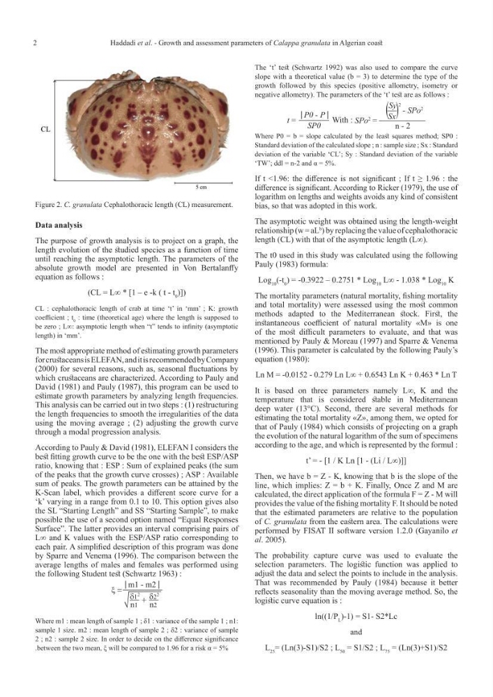
Figure 2. C. granulata Cephalothoracic length (CL) measurement.
Data analysis
The purpose of growth analysis is to project on a graph, the
length evolution of the studied species as a function of time
until reaching the asymptotic length. The parameters of the
absolute growth model are presented in Von Bertalanffy
equation as follows :
(CL = L∞ * [1 – e -k ( t - t 0 )])
CL : cephalothoracic length of crab at time ‘t’ in ‘mm’ ; K: growth
coefficient ; t 0 : time (theoretical age) where the length is supposed to
be zero ; L∞: asymptotic length when “t” tends to infinity (asymptotic
length) in ‘mm’.
The most appropriate method of estimating growth parameters
for crustaceans is ELEFAN, and it is recommended by Company
(2000) for several reasons, such as, seasonal fluctuations by
which crustaceans are characterized. According to Pauly and
David (1981) and Pauly (1987), this program can be used to
estimate growth parameters by analyzing length frequencies.
This analysis can be carried out in two steps : (1) restructuring
the length frequencies to smooth the irregularities of the data
using the moving average ; (2) adjusting the growth curve
through a modal progression analysis.
According to Pauly & David (1981), ELEFAN I considers the
best fitting growth curve to be the one with the best ESP/ASP
ratio, knowing that : ESP : Sum of explained peaks (the sum
of the peaks that the growth curve crosses) ; ASP : Available
sum of peaks. The growth parameters can be attained by the
K-Scan label, which provides a different score curve for a
‘k’ varying in a range from 0.1 to 10. This option gives also
the SL “Starting Length” and SS “Starting Sample”, to make
possible the use of a second option named “Equal Responses
Surface”. The latter provides an interval comprising pairs of
L∞ and K values with the ESP/ASP ratio corresponding to
each pair. A simplified description of this program was done
by Sparre and Venema (1996). The comparison between the
average lengths of males and females was performed using
the following Student test (Schwartz 1963) :
m1 - m2
ξ =
+
δ1
2
n1
δ2
2
n2
Where m1 : mean length of sample 1 ; δ1 : variance of the sample 1 ; n1:
sample 1 size. m2 : mean length of sample 2 ; δ2 : variance of sample
2 ; n2 : sample 2 size. In order to decide on the difference significance
.between the two mean, ξ will be compared to 1.96 for a risk α = 5%
The ‘t’ test (Schwartz 1992) was also used to compare the curve
slope with a theoretical value (b = 3) to determine the type of the
growth followed by this species (positive allometry, isometry or
negative allometry). The parameters of the ‘t’ test are as follows :
P0 - P
t = SP0
With :
- SPo
2
SPo
2
=
n - 2
(
Sy
Sx )
2
Where P0 = b = slope calculated by the least squares method; SP0 :
Standard deviation of the calculated slope ; n : sample size ; Sx : Standard
deviation of the variable ‘CL’; Sy : Standard deviation of the variable
‘TW’; ddl = n-2 and α = 5%.
If t <1.96: the difference is not significant ; If t ≥ 1.96 : the
difference is significant. According to Ricker (1979), the use of
logarithm on lengths and weights avoids any kind of consistent
bias, so that was adopted in this work.
The asymptotic weight was obtained using the length-weight
relationship (w = aL
b
) by replacing the value of cephalothoracic
length (CL) with that of the asymptotic length (L∞).
The t0 used in this study was calculated using the following
Pauly (1983) formula:
Log 10 (-t 0 ) = -0.3922 – 0.2751 * Log 10 L∞ - 1.038 * Log 10 K
The mortality parameters (natural mortality, fishing mortality
and total mortality) were assessed using the most common
methods adapted to the Mediterranean stock. First, the
instantaneous coefficient of natural mortality «M» is one
of the most difficult parameters to evaluate, and that was
mentioned by Pauly & Moreau (1997) and Sparre & Venema
(1996). This parameter is calculated by the following Pauly’s
equation (1980):
Ln M = -0.0152 - 0.279 Ln L∞ + 0.6543 Ln K + 0.463 * Ln T
It is based on three parameters namely L∞, K and the
temperature that is considered stable in Mediterranean
deep water (13°C). Second, there are several methods for
estimating the total mortality «Z», among them, we opted for
that of Pauly (1984) which consists of projecting on a graph
the evolution of the natural logarithm of the sum of specimens
according to the age, and which is represented by the formul :
t’ = - [1 / K Ln [1 - (Li / L∞)]]
Then, we have b = Z - K, knowing that b is the slope of the
line, which implies: Z = b + K. Finally, Once Z and M are
calculated, the direct application of the formula F = Z - M will
provides the value of the fishing mortality F. It should be noted
that the estimated parameters are relative to the population
of C. granulata from the eastern area. The calculations were
performed by FISAT II software version 1.2.0 (Gayanilo et
al. 2005).
The probability capture curve was used to evaluate the
selection parameters. The logistic function was applied to
adjust the data and select the points to include in the analysis.
That was recommended by Pauly (1984) because it better
reflects seasonality than the moving average method. So, the
logistic curve equation is :
ln((1/P L )-1) = S1- S2*Lc
and
L 25 = (Ln(3)-S1)/S2 ; L 50 = S1/S2 ; L 75 = (Ln(3)+S1)/S2
Haddadi et al. - Growth and assessment parameters of Calappa granulata in Algerian coast
Figure 2. C. granulata Cephalothoracic length (CL) measurement.
Data analysis
The purpose of growth analysis is to project on a graph, the
length evolution of the studied species as a function of time
until reaching the asymptotic length. The parameters of the
absolute growth model are presented in Von Bertalanffy
equation as follows :
(CL = L∞ * [1 – e -k ( t - t 0 )])
CL : cephalothoracic length of crab at time ‘t’ in ‘mm’ ; K: growth
coefficient ; t 0 : time (theoretical age) where the length is supposed to
be zero ; L∞: asymptotic length when “t” tends to infinity (asymptotic
length) in ‘mm’.
The most appropriate method of estimating growth parameters
for crustaceans is ELEFAN, and it is recommended by Company
(2000) for several reasons, such as, seasonal fluctuations by
which crustaceans are characterized. According to Pauly and
David (1981) and Pauly (1987), this program can be used to
estimate growth parameters by analyzing length frequencies.
This analysis can be carried out in two steps : (1) restructuring
the length frequencies to smooth the irregularities of the data
using the moving average ; (2) adjusting the growth curve
through a modal progression analysis.
According to Pauly & David (1981), ELEFAN I considers the
best fitting growth curve to be the one with the best ESP/ASP
ratio, knowing that : ESP : Sum of explained peaks (the sum
of the peaks that the growth curve crosses) ; ASP : Available
sum of peaks. The growth parameters can be attained by the
K-Scan label, which provides a different score curve for a
‘k’ varying in a range from 0.1 to 10. This option gives also
the SL “Starting Length” and SS “Starting Sample”, to make
possible the use of a second option named “Equal Responses
Surface”. The latter provides an interval comprising pairs of
L∞ and K values with the ESP/ASP ratio corresponding to
each pair. A simplified description of this program was done
by Sparre and Venema (1996). The comparison between the
average lengths of males and females was performed using
the following Student test (Schwartz 1963) :
m1 - m2
ξ =
+
δ1
2
n1
δ2
2
n2
Where m1 : mean length of sample 1 ; δ1 : variance of the sample 1 ; n1:
sample 1 size. m2 : mean length of sample 2 ; δ2 : variance of sample
2 ; n2 : sample 2 size. In order to decide on the difference significance
.between the two mean, ξ will be compared to 1.96 for a risk α = 5%
The ‘t’ test (Schwartz 1992) was also used to compare the curve
slope with a theoretical value (b = 3) to determine the type of the
growth followed by this species (positive allometry, isometry or
negative allometry). The parameters of the ‘t’ test are as follows :
P0 - P
t = SP0
With :
- SPo
2
SPo
2
=
n - 2
(
Sy
Sx )
2
Where P0 = b = slope calculated by the least squares method; SP0 :
Standard deviation of the calculated slope ; n : sample size ; Sx : Standard
deviation of the variable ‘CL’; Sy : Standard deviation of the variable
‘TW’; ddl = n-2 and α = 5%.
If t <1.96: the difference is not significant ; If t ≥ 1.96 : the
difference is significant. According to Ricker (1979), the use of
logarithm on lengths and weights avoids any kind of consistent
bias, so that was adopted in this work.
The asymptotic weight was obtained using the length-weight
relationship (w = aL
b
) by replacing the value of cephalothoracic
length (CL) with that of the asymptotic length (L∞).
The t0 used in this study was calculated using the following
Pauly (1983) formula:
Log 10 (-t 0 ) = -0.3922 – 0.2751 * Log 10 L∞ - 1.038 * Log 10 K
The mortality parameters (natural mortality, fishing mortality
and total mortality) were assessed using the most common
methods adapted to the Mediterranean stock. First, the
instantaneous coefficient of natural mortality «M» is one
of the most difficult parameters to evaluate, and that was
mentioned by Pauly & Moreau (1997) and Sparre & Venema
(1996). This parameter is calculated by the following Pauly’s
equation (1980):
Ln M = -0.0152 - 0.279 Ln L∞ + 0.6543 Ln K + 0.463 * Ln T
It is based on three parameters namely L∞, K and the
temperature that is considered stable in Mediterranean
deep water (13°C). Second, there are several methods for
estimating the total mortality «Z», among them, we opted for
that of Pauly (1984) which consists of projecting on a graph
the evolution of the natural logarithm of the sum of specimens
according to the age, and which is represented by the formul :
t’ = - [1 / K Ln [1 - (Li / L∞)]]
Then, we have b = Z - K, knowing that b is the slope of the
line, which implies: Z = b + K. Finally, Once Z and M are
calculated, the direct application of the formula F = Z - M will
provides the value of the fishing mortality F. It should be noted
that the estimated parameters are relative to the population
of C. granulata from the eastern area. The calculations were
performed by FISAT II software version 1.2.0 (Gayanilo et
al. 2005).
The probability capture curve was used to evaluate the
selection parameters. The logistic function was applied to
adjust the data and select the points to include in the analysis.
That was recommended by Pauly (1984) because it better
reflects seasonality than the moving average method. So, the
logistic curve equation is :
ln((1/P L )-1) = S1- S2*Lc
and
L 25 = (Ln(3)-S1)/S2 ; L 50 = S1/S2 ; L 75 = (Ln(3)+S1)/S2