

for all subsequent layers, so that contributions from above-ground features are
gradually removed from the coefficients.
The surface gradient along transitions between ground and nonground points is
assumed higher than the maximum terrain slope. This is generally the case for
features of sizes much larger than the average sampling distance of Lidar data. In
contrast, small trees, cars, or other low features embedded in data sets with average
point distance greater than 1 m tend to produce smaller gradient values than some
terrain features. Ground/nonground transitions are detected by comparing the local
gradient z
q;k
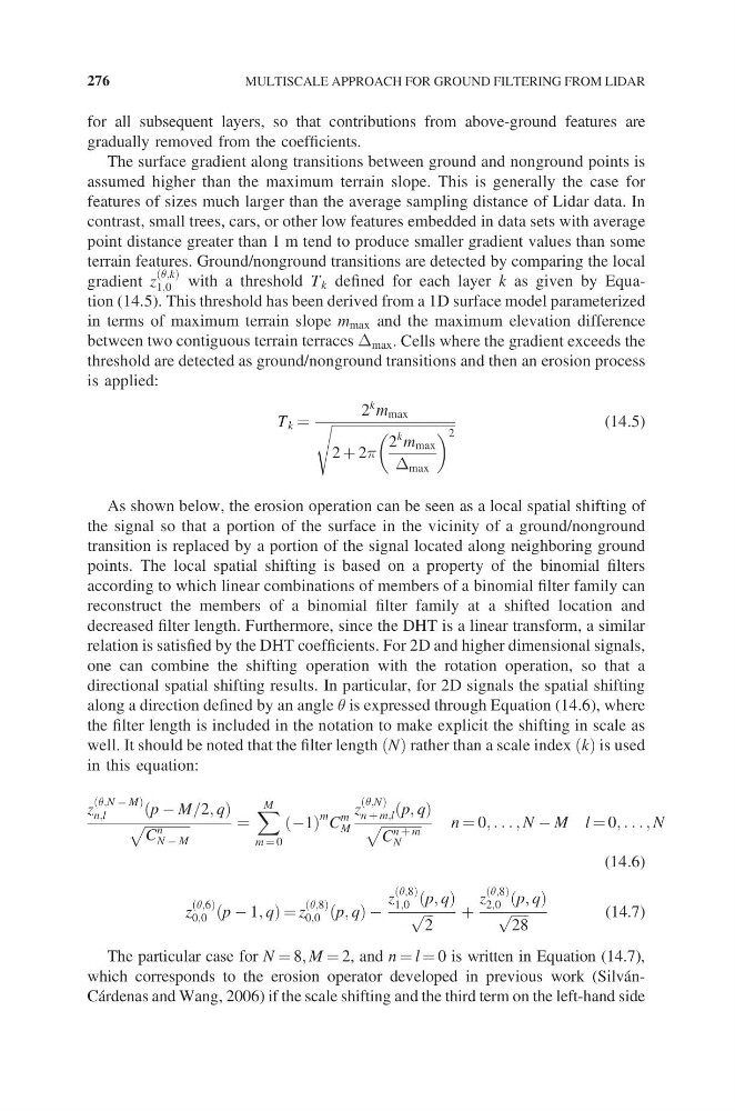
1;0 with a threshold T k defined for each layer k as given by Equation (14.5). This threshold has been derived from a 1D surface model parameterized
in terms of maximum terrain slope m max and the maximum elevation difference
between two contiguous terrain terraces D max . Cells where the gradient exceeds the
threshold are detected as ground/nonground transitions and then an erosion process
is applied:
T k =
2
k m max
ffiffiffiffiffiffiffiffiffiffiffiffiffiffiffiffiffiffiffiffiffiffiffiffiffiffiffiffiffiffiffiffiffiffiffiffi
2 + 2p
2
k m max
D max
2
s
(14.5)
As shown below, the erosion operation can be seen as a local spatial shifting of
the signal so that a portion of the surface in the vicinity of a ground/nonground
transition is replaced by a portion of the signal located along neighboring ground
points. The local spatial shifting is based on a property of the binomial filters
according to which linear combinations of members of a binomial filter family can
reconstruct the members of a binomial filter family at a shifted location and
decreased filter length. Furthermore, since the DHT is a linear transform, a similar
relation is satisfied by the DHT coefficients. For 2D and higher dimensional signals,
one can combine the shifting operation with the rotation operation, so that a
directional spatial shifting results. In particular, for 2D signals the spatial shifting
along a direction defined by an angle q is expressed through Equation (14.6), where
the filter length is included in the notation to make explicit the shifting in scale as
well. It should be noted that the filter length N rather than a scale index k is used
in this equation:
z
q;N − M
n;l
p − M=2; q
ffiffiffiffiffiffiffiffiffiffiffiffiffi
C
n
N − M
p
=
X M
m = 0
−1
m C
m
M
z
q;N
n + m;l p; q
ffiffiffiffiffiffiffiffiffiffiffi ffi
C
n + m
N
p
n = 0; . . . ; N − M l= 0; . . . ; N
(14.6)
z
q;6
0;0 p − 1; q = z
q;8
0;0 p; q −
z
q;8
1;0 p; q
ffiffi ffi
2
p
+
z
q;8
2;0 p; q
ffiffiffiffiffi
28
p
(14.7)
The particular case for N = 8; M = 2, and n = l = 0 is written in Equation (14.7),
which corresponds to the erosion operator developed in previous work (SilvánCárdenas and Wang, 2006) if the scale shifting and the third term on the left-hand side
276
MULTISCALE APPROACH FOR GROUND FILTERING FROM LIDAR
gradually removed from the coefficients.
The surface gradient along transitions between ground and nonground points is
assumed higher than the maximum terrain slope. This is generally the case for
features of sizes much larger than the average sampling distance of Lidar data. In
contrast, small trees, cars, or other low features embedded in data sets with average
point distance greater than 1 m tend to produce smaller gradient values than some
terrain features. Ground/nonground transitions are detected by comparing the local
gradient z
q;k
1;0 with a threshold T k defined for each layer k as given by Equation (14.5). This threshold has been derived from a 1D surface model parameterized
in terms of maximum terrain slope m max and the maximum elevation difference
between two contiguous terrain terraces D max . Cells where the gradient exceeds the
threshold are detected as ground/nonground transitions and then an erosion process
is applied:
T k =
2
k m max
ffiffiffiffiffiffiffiffiffiffiffiffiffiffiffiffiffiffiffiffiffiffiffiffiffiffiffiffiffiffiffiffiffiffiffiffi
2 + 2p
2
k m max
D max
2
s
(14.5)
As shown below, the erosion operation can be seen as a local spatial shifting of
the signal so that a portion of the surface in the vicinity of a ground/nonground
transition is replaced by a portion of the signal located along neighboring ground
points. The local spatial shifting is based on a property of the binomial filters
according to which linear combinations of members of a binomial filter family can
reconstruct the members of a binomial filter family at a shifted location and
decreased filter length. Furthermore, since the DHT is a linear transform, a similar
relation is satisfied by the DHT coefficients. For 2D and higher dimensional signals,
one can combine the shifting operation with the rotation operation, so that a
directional spatial shifting results. In particular, for 2D signals the spatial shifting
along a direction defined by an angle q is expressed through Equation (14.6), where
the filter length is included in the notation to make explicit the shifting in scale as
well. It should be noted that the filter length N rather than a scale index k is used
in this equation:
z
q;N − M
n;l
p − M=2; q
ffiffiffiffiffiffiffiffiffiffiffiffiffi
C
n
N − M
p
=
X M
m = 0
−1
m C
m
M
z
q;N
n + m;l p; q
ffiffiffiffiffiffiffiffiffiffiffi ffi
C
n + m
N
p
n = 0; . . . ; N − M l= 0; . . . ; N
(14.6)
z
q;6
0;0 p − 1; q = z
q;8
0;0 p; q −
z
q;8
1;0 p; q
ffiffi ffi
2
p
+
z
q;8
2;0 p; q
ffiffiffiffiffi
28
p
(14.7)
The particular case for N = 8; M = 2, and n = l = 0 is written in Equation (14.7),
which corresponds to the erosion operator developed in previous work (SilvánCárdenas and Wang, 2006) if the scale shifting and the third term on the left-hand side
276
MULTISCALE APPROACH FOR GROUND FILTERING FROM LIDAR