

case presented here, the rotation angle was set to the orientation of the local
gradient, which can be directly computed from the first-order coefficients as
expressed in Equation (14.1):
q = arctan
z
k
0;1
z
k
1;0
!
(14.1)
z
k;q
0;1 = 0
z
k;q
1;0 =
ffiffiffiffiffiffiffiffiffiffiffiffiffiffiffiffiffiffiffiffiffiffiffiffiffiffiffiffiffiffiffiffiffi ffi
z
k
1;0
2 + z
k
0;1
2
r
(14.2)
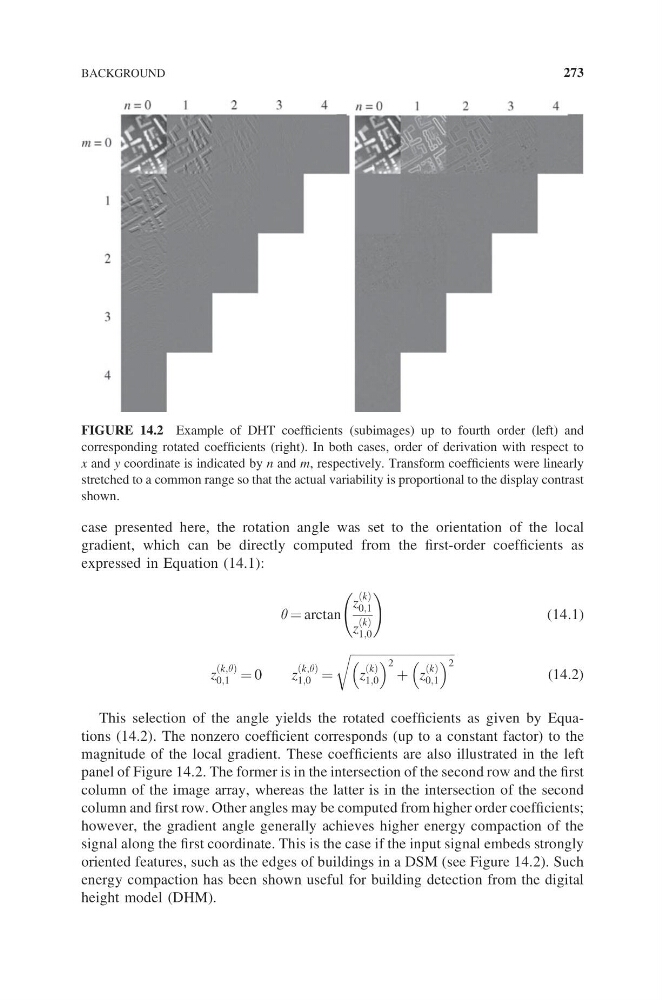
This selection of the angle yields the rotated coefficients as given by Equations (14.2). The nonzero coefficient corresponds (up to a constant factor) to the
magnitude of the local gradient. These coefficients are also illustrated in the left
panel of Figure 14.2. The former is in the intersection of the second row and the first
column of the image array, whereas the latter is in the intersection of the second
column and first row. Other angles may be computed from higher order coefficients;
however, the gradient angle generally achieves higher energy compaction of the
signal along the first coordinate. This is the case if the input signal embeds strongly
oriented features, such as the edges of buildings in a DSM (see Figure 14.2). Such
energy compaction has been shown useful for building detection from the digital
height model (DHM).
FIGURE 14.2 Example of DHT coefficients (subimages) up to fourth order (left) and
corresponding rotated coefficients (right). In both cases, order of derivation with respect to
x and y coordinate is indicated by n and m, respectively. Transform coefficients were linearly
stretched to a common range so that the actual variability is proportional to the display contrast
shown.
BACKGROUND
273
gradient, which can be directly computed from the first-order coefficients as
expressed in Equation (14.1):
q = arctan
z
k
0;1
z
k
1;0
!
(14.1)
z
k;q
0;1 = 0
z
k;q
1;0 =
ffiffiffiffiffiffiffiffiffiffiffiffiffiffiffiffiffiffiffiffiffiffiffiffiffiffiffiffiffiffiffiffiffi ffi
z
k
1;0
2 + z
k
0;1
2
r
(14.2)
This selection of the angle yields the rotated coefficients as given by Equations (14.2). The nonzero coefficient corresponds (up to a constant factor) to the
magnitude of the local gradient. These coefficients are also illustrated in the left
panel of Figure 14.2. The former is in the intersection of the second row and the first
column of the image array, whereas the latter is in the intersection of the second
column and first row. Other angles may be computed from higher order coefficients;
however, the gradient angle generally achieves higher energy compaction of the
signal along the first coordinate. This is the case if the input signal embeds strongly
oriented features, such as the edges of buildings in a DSM (see Figure 14.2). Such
energy compaction has been shown useful for building detection from the digital
height model (DHM).
FIGURE 14.2 Example of DHT coefficients (subimages) up to fourth order (left) and
corresponding rotated coefficients (right). In both cases, order of derivation with respect to
x and y coordinate is indicated by n and m, respectively. Transform coefficients were linearly
stretched to a common range so that the actual variability is proportional to the display contrast
shown.
BACKGROUND
273