

70
Basic biogeography: estimating biodiversity and mapping nature
Our second example made use of excellent survey
data for a well - known group: British birds. In this
study, Ara ú jo et al . (2005b) used four different modelling methods combined with a number of different
parameterizations, providing 16 alternative models
for each species, to simulate the distributions of 116
breeding bird species for two periods. Despite the fact
that they had generated mostly adequate statistical
models for the period 1967 – 1972, when these ‘ time 1 ’
models were used to generate predictions for the distributions of the same species using the climate data for
cells in the data set when generating the model, and
then testing the ability of the model to predict the
species distribution for the test subset. Scientists use
this same modelling approach to generate projections
not only of current distributions, but of future distributions as a function of environmental (and especially
climate change). As Whitfi eld (2009) recently commented, ‘ Such models are among the main tools in
efforts to predict and plan for the biological effects of
climate change. And because their predictions can be
displayed as intuitive and dramatic maps, they have a
psychological power beyond most scientifi c graphics. ’
Modelling the dispersal capacity of the species and its
ability to keep up with climate change or to ‘ jump disperse ’ between widely separated cells of suitable climate
is a particularly diffi cult challenge. It is one that has
typically been either ignored or addressed by contrasting the effect on the modelled outcome of no dispersal,
on the one hand, versus free dispersal on the other.
The use of BEMs in the context of climate change is
of particular interest and will be discussed further in
Chapter 9 . Here we give just two examples that illustrate two key pitfalls of these approaches. The fi rst
pitfall is that data of dubious validity can still lead to
good models, and the second is that even good model
fi ts are no guarantee of time - transferability of models.
Lozier et al . (2009) provide an analysis for a cryptozoogeographical taxon, the North American bigfoot or
sasquatch. This species is so cryptic that its status
belongs more to the realm of myth and legend rather
than to the Linnean and Wallacean shortfalls. However,
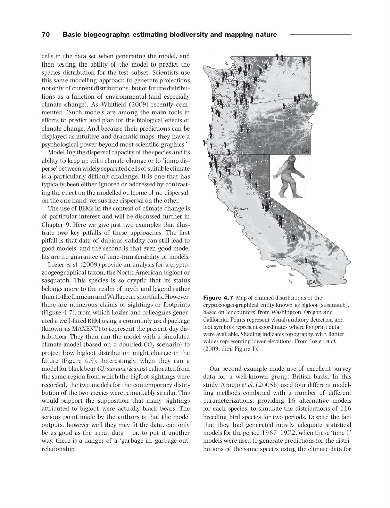
there are numerous claims of sightings or footprints
(Figure 4.7 ), from which Lozier and colleagues generated a well - fi tted BEM using a commonly used package
(known as MAXENT) to represent the present - day distribution. They then ran the model with a simulated
climate model (based on a doubled CO 2 scenario) to
project how bigfoot distribution might change in the
future (Figure 4.8 ). Interestingly, when they ran a
model for black bear ( Ursus americanus ) calibrated from
the same region from which the bigfoot sightings were
recorded, the two models for the contemporary distribution of the two species were remarkably similar. This
would support the supposition that many sightings
attributed to bigfoot were actually black bears. The
serious point made by the authors is that the model
outputs, however well they may fi t the data, can only
be as good as the input data – or, to put it another
way, there is a danger of a ‘ garbage in, garbage out ’
relationship.
Figure 4.7 Map of claimed distributions of the
cryptozoogeographical entity known as bigfoot (sasquatch),
based on ‘ encounters ’ from Washington, Oregon and
California. Points represent visual/auditory detection and
foot symbols represent coordinates where footprint data
were available. Shading indicates topography, with lighter
values representing lower elevations. From Lozier et al.
( 2009 , their Figure 1).
Basic biogeography: estimating biodiversity and mapping nature
Our second example made use of excellent survey
data for a well - known group: British birds. In this
study, Ara ú jo et al . (2005b) used four different modelling methods combined with a number of different
parameterizations, providing 16 alternative models
for each species, to simulate the distributions of 116
breeding bird species for two periods. Despite the fact
that they had generated mostly adequate statistical
models for the period 1967 – 1972, when these ‘ time 1 ’
models were used to generate predictions for the distributions of the same species using the climate data for
cells in the data set when generating the model, and
then testing the ability of the model to predict the
species distribution for the test subset. Scientists use
this same modelling approach to generate projections
not only of current distributions, but of future distributions as a function of environmental (and especially
climate change). As Whitfi eld (2009) recently commented, ‘ Such models are among the main tools in
efforts to predict and plan for the biological effects of
climate change. And because their predictions can be
displayed as intuitive and dramatic maps, they have a
psychological power beyond most scientifi c graphics. ’
Modelling the dispersal capacity of the species and its
ability to keep up with climate change or to ‘ jump disperse ’ between widely separated cells of suitable climate
is a particularly diffi cult challenge. It is one that has
typically been either ignored or addressed by contrasting the effect on the modelled outcome of no dispersal,
on the one hand, versus free dispersal on the other.
The use of BEMs in the context of climate change is
of particular interest and will be discussed further in
Chapter 9 . Here we give just two examples that illustrate two key pitfalls of these approaches. The fi rst
pitfall is that data of dubious validity can still lead to
good models, and the second is that even good model
fi ts are no guarantee of time - transferability of models.
Lozier et al . (2009) provide an analysis for a cryptozoogeographical taxon, the North American bigfoot or
sasquatch. This species is so cryptic that its status
belongs more to the realm of myth and legend rather
than to the Linnean and Wallacean shortfalls. However,
there are numerous claims of sightings or footprints
(Figure 4.7 ), from which Lozier and colleagues generated a well - fi tted BEM using a commonly used package
(known as MAXENT) to represent the present - day distribution. They then ran the model with a simulated
climate model (based on a doubled CO 2 scenario) to
project how bigfoot distribution might change in the
future (Figure 4.8 ). Interestingly, when they ran a
model for black bear ( Ursus americanus ) calibrated from
the same region from which the bigfoot sightings were
recorded, the two models for the contemporary distribution of the two species were remarkably similar. This
would support the supposition that many sightings
attributed to bigfoot were actually black bears. The
serious point made by the authors is that the model
outputs, however well they may fi t the data, can only
be as good as the input data – or, to put it another
way, there is a danger of a ‘ garbage in, garbage out ’
relationship.
Figure 4.7 Map of claimed distributions of the
cryptozoogeographical entity known as bigfoot (sasquatch),
based on ‘ encounters ’ from Washington, Oregon and
California. Points represent visual/auditory detection and
foot symbols represent coordinates where footprint data
were available. Shading indicates topography, with lighter
values representing lower elevations. From Lozier et al.
( 2009 , their Figure 1).