

Environmental change
609
climate change can be abrupt and, as a result, a response is triggered. This response,
although short, can be opposite to the curve of soil loss of Langbein and Schumm (1958).
This author (Knox) pointed out that if there is an intense and maintained increase in
precipitation, this causes erosion of the channel and a rise in slope gradient (Figure 23.7C).
Therefore, in this short period of time an important increase in the loss of soil is also
produced, followed by a fall (Figure 23.7D). Nevertheless, these fluctuations are difficult to
distinguish from the effect of large flooding with long return period (Chorley et al., 1984).
3. Future climate and the greenhouse effect
The study of the climate trend is nowadays the purpose of many researches, as a result of
the increased warming predicted by scientists due to the effect of greenhouse gases. These
gases are water vapour, carbon dioxide, nitrous oxide, methane, and chlorofluorocarbonates. They have increased during the last decades, affecting the global climate. The most
significant effect is due to the rise of carbon dioxide produced by the combustion of
an ever-increasing quantity of coal, petroleum, and other fossil combustibles, as well as
woodcutting and forest fires. The CO2 is almost transparent to short-wave solar radiation
and absorbs a major part of the long wave. Therefore, it is one of the factors that produce a
greenhouse effect, raising the temperature of the Earth's surface and lower atmosphere.
Thus an increase in the quantity of CO2 leads to global warming (Budyko, 1982).
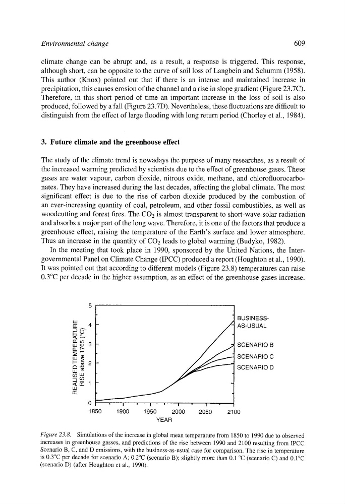
In the meeting that took place in 1990, sponsored by the United Nations, the Intergovernmental Panel on Climate Change (IPCC) produced a report (Houghton et al., 1990).
It was pointed out that according to different models (Figure 23.8) temperatures can raise
0.3~ per decade in the higher assumption, as an effect of the greenhouse gases increase.
uJ
n"
4 -
v
rru3
uj~3
13_ v..I--- o
o-~ 2
LM
.
J~
rr
.
0 -1850
1900
1950
2000
2050
2100
YEAR
BUSINESSAS-USUAL
SCENARIO B
SCENARIO C
SCENARIO D
Figure 23.8. Simulations of the increase in global mean temperature from 1850 to 1990 due to observed
increases in greenhouse gasses, and predictions of the rise between 1990 and 2100 resulting from IPCC
Scenario B, C, and D emissions, with the business-as-usual case for comparison. The rise in temperature
is 0.3~ per decade for scenario A; 0.2~ (scenario B); slightly more than 0.1 ~ (scenario C) and 0.1~
(scenario D) (after Houghton et al., 1990).