

Optical Spectroscopy Instrumentation Design
183
5.4.18 Correcting Excitation Signal Channels
Correction can be divided into two types:
To use a previously measured correction file, or
•
To actively monitor the light intensity during the measurement and make the correction
•
live
In the first method it is important to know the spectral response of the reference detector.
This can be measured separately using a calibrated tungsten light source and the monochromator under test in the system if the spectral response of the reference detector is not
already known. Normally, the correction file, Ex Cor
−
( )
λ , is normalized to give a range
from 0 to 1, where the peak intensity is 1 and the minimum fluorescence intensity is 0.
If the measured spectrum is S m λ
( ) then the corrected sample file Sc Ex
S m
−
( ) = ( ) /
λ
λ
Ex Cor
−
( )
λ .
It is imperative that the Ex Cor
−
( )
λ file should be determined under the same bandpass
parameters as the sample measurement. More important is to ensure that the step size for
each file is the same and that the Ex Cor
−
( )
λ file covers at least the same spectral region
as the measurement, S m λ
( ). If the step sizes are different between these two files then an
interpolation needs to be ascertained in order to fill in the “missing data points.” For example: if Ex Cor
−
( )
λ is measured with 2 nm step size then there is a data point every 2 nm. If
the sample S m λ
( ) is measured at 0.5 nm step size over the same spectral range then there
are four times as many data points in the S m file as there are in the Ex Cor
−
file, meaning
that a simple division of one file with the other becomes problematic. This issue is negated
by interpolating between the data points in the Ex Cor
−
file to make an equivalent number
of data points of the same file length. Often this interpolation is a straight line between
the existing points, but more complex functions are also sometimes used. This problem
applies equally to using a reference detector and also to the emission channel correction.
In some ways the process of using the reference detector is quite similar to that of the
correction file. The main difference is that we make the correction measurement “live”
with every excitation scan. We need to know what the spectral response of the reference
detector is so that we can correct for the reference detector itself. If the spectral response of
the reference detector is, Ref Det
−
( )
λ , and the measured signal from the reference detector
is Ref Sig
−
( )
λ , then the Ex Cor
−
( )
λ = Ref Sig
−
( )
λ / Ref Det
−
( ).
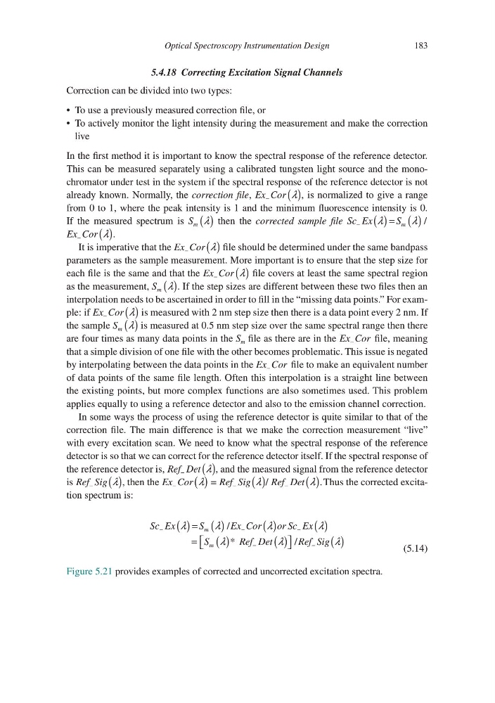
λ Thus the corrected excitation spectrum is:
Sc Ex
S
Ex Cor
or Sc Ex
S
R ef Det
m
m
−
−
−
−
( ) = ( )
( )
( )
=
( )
/
*
λ
λ
λ
λ
λ
λ
( )
( )
−
/Ref Sig λ
(5.14)
Figure 5.21 provides examples of corrected and uncorrected excitation spectra.
183
5.4.18 Correcting Excitation Signal Channels
Correction can be divided into two types:
To use a previously measured correction file, or
•
To actively monitor the light intensity during the measurement and make the correction
•
live
In the first method it is important to know the spectral response of the reference detector.
This can be measured separately using a calibrated tungsten light source and the monochromator under test in the system if the spectral response of the reference detector is not
already known. Normally, the correction file, Ex Cor
−
( )
λ , is normalized to give a range
from 0 to 1, where the peak intensity is 1 and the minimum fluorescence intensity is 0.
If the measured spectrum is S m λ
( ) then the corrected sample file Sc Ex
S m
−
( ) = ( ) /
λ
λ
Ex Cor
−
( )
λ .
It is imperative that the Ex Cor
−
( )
λ file should be determined under the same bandpass
parameters as the sample measurement. More important is to ensure that the step size for
each file is the same and that the Ex Cor
−
( )
λ file covers at least the same spectral region
as the measurement, S m λ
( ). If the step sizes are different between these two files then an
interpolation needs to be ascertained in order to fill in the “missing data points.” For example: if Ex Cor
−
( )
λ is measured with 2 nm step size then there is a data point every 2 nm. If
the sample S m λ
( ) is measured at 0.5 nm step size over the same spectral range then there
are four times as many data points in the S m file as there are in the Ex Cor
−
file, meaning
that a simple division of one file with the other becomes problematic. This issue is negated
by interpolating between the data points in the Ex Cor
−
file to make an equivalent number
of data points of the same file length. Often this interpolation is a straight line between
the existing points, but more complex functions are also sometimes used. This problem
applies equally to using a reference detector and also to the emission channel correction.
In some ways the process of using the reference detector is quite similar to that of the
correction file. The main difference is that we make the correction measurement “live”
with every excitation scan. We need to know what the spectral response of the reference
detector is so that we can correct for the reference detector itself. If the spectral response of
the reference detector is, Ref Det
−
( )
λ , and the measured signal from the reference detector
is Ref Sig
−
( )
λ , then the Ex Cor
−
( )
λ = Ref Sig
−
( )
λ / Ref Det
−
( ).
λ Thus the corrected excitation spectrum is:
Sc Ex
S
Ex Cor
or Sc Ex
S
R ef Det
m
m
−
−
−
−
( ) = ( )
( )
( )
=
( )
/
*
λ
λ
λ
λ
λ
λ
( )
( )
−
/Ref Sig λ
(5.14)
Figure 5.21 provides examples of corrected and uncorrected excitation spectra.