

Gilchrist and Reynolds
172
Application standards – such as spectrally matched and known fluorophores whose prop•
erties are close to those of the samples being measured.
In many cases, quantitative fluorescence assessment often consists of undertaking some
intensity calibration of the instrument response with respect to the concentration of some
“standard” fluorophore in a certain solvent. These titration type experiments are a common
way to “calibrate” an instrument but they rely critically on very precise determinations of
the fluorophore purity, solvent purity, initial concentration determinations, dilutions methods, pH and temperature control, and so forth. The whole process is fraught with possible
sources of both random and systematic errors and of course is applicable only to that particular instrument at that time.
In reality, the long-term stability of an instrument is one of the key concerns of both the
manufacturer and the user. Thus, day-to-day and even instrument-to-instrument validation is
needed. One of the best known methods to achieve this is to undertake the so-called “water
Table 5.5. Measurement and analysis of signal-to-noise using the water Raman test
Measurement conditions
Excitation:
Emission scan:
Integration time:
λ exc = 350 nm, with Δλ exc = 5 nm
370 < λ em < 460 nm, with Δλ em =5nm, and scan
in δλ=1 nm steps
1 s per step
Analysis method
Signal = (peak signal at 397 nm) – (Average back ground signal)
SNR: Signal/background noise in range 450–460 nm
370 380 390 400 410
Wavelength (nm)
Intensity
420 430 430
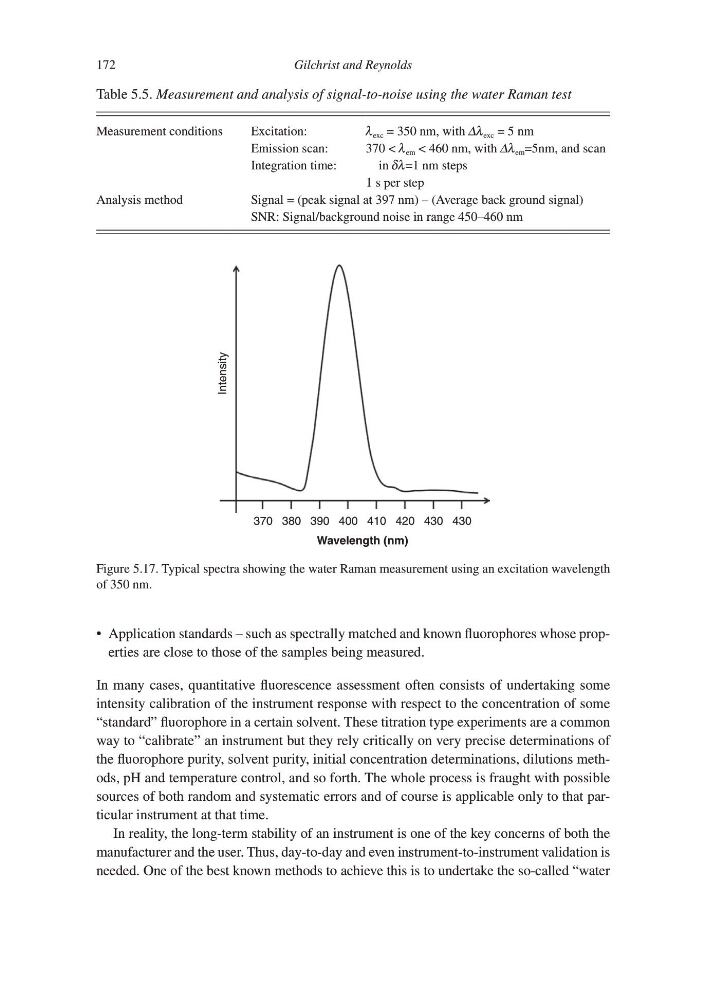
Figure 5.17. Typical spectra showing the water Raman measurement using an excitation wavelength
of 350 nm.
172
Application standards – such as spectrally matched and known fluorophores whose prop•
erties are close to those of the samples being measured.
In many cases, quantitative fluorescence assessment often consists of undertaking some
intensity calibration of the instrument response with respect to the concentration of some
“standard” fluorophore in a certain solvent. These titration type experiments are a common
way to “calibrate” an instrument but they rely critically on very precise determinations of
the fluorophore purity, solvent purity, initial concentration determinations, dilutions methods, pH and temperature control, and so forth. The whole process is fraught with possible
sources of both random and systematic errors and of course is applicable only to that particular instrument at that time.
In reality, the long-term stability of an instrument is one of the key concerns of both the
manufacturer and the user. Thus, day-to-day and even instrument-to-instrument validation is
needed. One of the best known methods to achieve this is to undertake the so-called “water
Table 5.5. Measurement and analysis of signal-to-noise using the water Raman test
Measurement conditions
Excitation:
Emission scan:
Integration time:
λ exc = 350 nm, with Δλ exc = 5 nm
370 < λ em < 460 nm, with Δλ em =5nm, and scan
in δλ=1 nm steps
1 s per step
Analysis method
Signal = (peak signal at 397 nm) – (Average back ground signal)
SNR: Signal/background noise in range 450–460 nm
370 380 390 400 410
Wavelength (nm)
Intensity
420 430 430
Figure 5.17. Typical spectra showing the water Raman measurement using an excitation wavelength
of 350 nm.