

47
4 The Economics of Eutrophication
• Stated preference methods: Where people are asked about
their willingness-to-pay for the environmental good or
service in question (see Hanemann 1994 for an overview,
and Diamond and Hausmann 1994 for a critical discussion).
Needless to say, the valuation estimates from such methods
may differ from the estimates obtained from modeling exercises or expert assessments. The main point here is that in
economics we would like to be able to compare the expected
benefits of environmental improvements with the costs of
obtaining these improvements.
4.3 Cost Effectiveness and Optimality
Cost effectiveness and optimality are key issues in environmental economics. A basic understanding of these concepts
is necessary to understand how economists reason on pollution issues in general and eutrophication in particular. Cost
effectiveness of an environmental policy is basically the
least cost way of reaching a certain environmental target, for
example, that emissions of nitrates to a receptor is not to exceed a certain level for a given time period. If faced with an
emission constraint, it is quite obvious that economic agents
(here polluters) would seek out the least cost way of not exceeding this constraint. A single polluter would hence implement the cheapest measure first, then the second cheapest
measure, and so forth until his or her emissions are just at or
below the permitted level. It is important to note that single
measures may not be uniformly cheapest—as a measure is
undertaken at increasing degrees; the costs associated with
single measures tend to increase. Hence, the polluter would
be looking at the combination of measures that yield the least
cost way of meeting the emission constraint.
To see this more clearly, consider a polluter who has four
ways of reducing his or her emissions of a pollutant from the
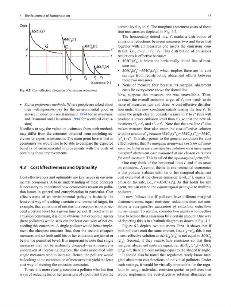
current level z 0 to z′. The marginal abatement costs of these
four measures are depicted in Fig. 4.2.
The horizontally dotted line, t′, marks a distribution of
emissions reductions between measures two and three that
together with all measures one meets the emissions constraint, i.e., z′ = z′ 1 + z′ 2 + z′ 3 . This distribution of emissions
reductions is effective because:
• MAC 1 ( z′ 1 ) is below the horizontally dotted line of measure one.
• MAC 2 ( z′ 2 ) = MAC 3 ( z′ 3 ), which implies there are no cost
savings from redistributing abatement efforts between
these two measures.
• None of measure four because its marginal abatement
costs lie everywhere above the dotted line.
Now, suppose that measure one was unavailable. Then,
to reach the overall emission target of z′, one needs to do
more of measures two and three. A cost-effective distribution under this new condition entails raising the line t′. To
make the graph clearer, consider a raise of t′ to t″ (this will
produce a lower emission level than z′), so that the new allocations z″ 2 > z′ 2 and z″ 3 > z′ 3 . Note that the new line t″ also
makes measure four also enter the cost-effective solution
with the amount z″ 4 because MAC 4 ( z″ 4 ) = MAC 2 ( z″ 2 ) = MAC 3
( z″ 3 ) = t″. This also points to the general condition for cost
effectiveness: that the marginal abatement costs for all measures included in the cost-effective solution must have equal
marginal abatement cost evaluated at the chosen emissions
for each measure. This is called the equimarginal principle.
One may think of the horizontal lines t′ and t″ as taxes
on emissions. A central theme in environmental economics
is that polluter i abates until his or her marginal abatement
cost evaluated at the chosen emission level, z′ i, equals the
emission tax rate, i.e., t′ = MAC i ( z′ i ). As this holds for any
agent, we can extend the equimarginal principle to multiple
polluters.
It now follows that if polluters have different marginal
abatement costs, equal emissions reductions does not constitute a cost-effective allocation of emissions reductions
across agents. To see this, consider two agents who together
have to reduce their emissions by a certain amount. One way
of depicting this is in a bathtub diagram as shown in Fig. 4.3.
Figure 4.3 depicts two situations. First, it shows that if
both polluters emit the same amount, i.e., z′ A = z′ B , this is not
a cost-effective solution as MAC A ( z′ A ) is not equal to MAC B
( z′ B ). Second, if they redistribute emissions so that their
marginal abatement costs are equal, i.e., MAC A ( z″ A ) = MAC B
( z″ B ) = t″, there are cost savings equal to the shaded triangle.
It should also be noted that regulators rarely know marginal abatement cost functions of individual polluters. Under
such settings, it would be virtually impossible for the regulator to assign individual emission quotas to polluters that
would implement the cost-effective solution illustrated in
Fig. 4.2 Cost-effective allocation of emissions reductions
4 The Economics of Eutrophication
• Stated preference methods: Where people are asked about
their willingness-to-pay for the environmental good or
service in question (see Hanemann 1994 for an overview,
and Diamond and Hausmann 1994 for a critical discussion).
Needless to say, the valuation estimates from such methods
may differ from the estimates obtained from modeling exercises or expert assessments. The main point here is that in
economics we would like to be able to compare the expected
benefits of environmental improvements with the costs of
obtaining these improvements.
4.3 Cost Effectiveness and Optimality
Cost effectiveness and optimality are key issues in environmental economics. A basic understanding of these concepts
is necessary to understand how economists reason on pollution issues in general and eutrophication in particular. Cost
effectiveness of an environmental policy is basically the
least cost way of reaching a certain environmental target, for
example, that emissions of nitrates to a receptor is not to exceed a certain level for a given time period. If faced with an
emission constraint, it is quite obvious that economic agents
(here polluters) would seek out the least cost way of not exceeding this constraint. A single polluter would hence implement the cheapest measure first, then the second cheapest
measure, and so forth until his or her emissions are just at or
below the permitted level. It is important to note that single
measures may not be uniformly cheapest—as a measure is
undertaken at increasing degrees; the costs associated with
single measures tend to increase. Hence, the polluter would
be looking at the combination of measures that yield the least
cost way of meeting the emission constraint.
To see this more clearly, consider a polluter who has four
ways of reducing his or her emissions of a pollutant from the
current level z 0 to z′. The marginal abatement costs of these
four measures are depicted in Fig. 4.2.
The horizontally dotted line, t′, marks a distribution of
emissions reductions between measures two and three that
together with all measures one meets the emissions constraint, i.e., z′ = z′ 1 + z′ 2 + z′ 3 . This distribution of emissions
reductions is effective because:
• MAC 1 ( z′ 1 ) is below the horizontally dotted line of measure one.
• MAC 2 ( z′ 2 ) = MAC 3 ( z′ 3 ), which implies there are no cost
savings from redistributing abatement efforts between
these two measures.
• None of measure four because its marginal abatement
costs lie everywhere above the dotted line.
Now, suppose that measure one was unavailable. Then,
to reach the overall emission target of z′, one needs to do
more of measures two and three. A cost-effective distribution under this new condition entails raising the line t′. To
make the graph clearer, consider a raise of t′ to t″ (this will
produce a lower emission level than z′), so that the new allocations z″ 2 > z′ 2 and z″ 3 > z′ 3 . Note that the new line t″ also
makes measure four also enter the cost-effective solution
with the amount z″ 4 because MAC 4 ( z″ 4 ) = MAC 2 ( z″ 2 ) = MAC 3
( z″ 3 ) = t″. This also points to the general condition for cost
effectiveness: that the marginal abatement costs for all measures included in the cost-effective solution must have equal
marginal abatement cost evaluated at the chosen emissions
for each measure. This is called the equimarginal principle.
One may think of the horizontal lines t′ and t″ as taxes
on emissions. A central theme in environmental economics
is that polluter i abates until his or her marginal abatement
cost evaluated at the chosen emission level, z′ i, equals the
emission tax rate, i.e., t′ = MAC i ( z′ i ). As this holds for any
agent, we can extend the equimarginal principle to multiple
polluters.
It now follows that if polluters have different marginal
abatement costs, equal emissions reductions does not constitute a cost-effective allocation of emissions reductions
across agents. To see this, consider two agents who together
have to reduce their emissions by a certain amount. One way
of depicting this is in a bathtub diagram as shown in Fig. 4.3.
Figure 4.3 depicts two situations. First, it shows that if
both polluters emit the same amount, i.e., z′ A = z′ B , this is not
a cost-effective solution as MAC A ( z′ A ) is not equal to MAC B
( z′ B ). Second, if they redistribute emissions so that their
marginal abatement costs are equal, i.e., MAC A ( z″ A ) = MAC B
( z″ B ) = t″, there are cost savings equal to the shaded triangle.
It should also be noted that regulators rarely know marginal abatement cost functions of individual polluters. Under
such settings, it would be virtually impossible for the regulator to assign individual emission quotas to polluters that
would implement the cost-effective solution illustrated in
Fig. 4.2 Cost-effective allocation of emissions reductions