

58
2: Raghuveer M. Rao, Manoj K. Arora
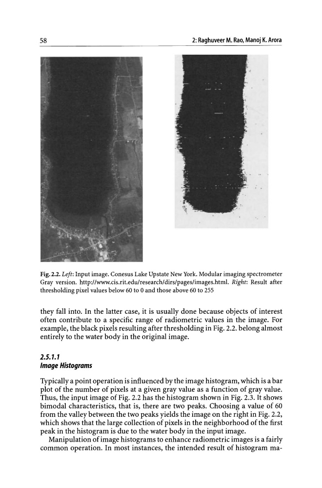
Fig. 2.2. Left: Input image. Conesus Lake Upstate New York. Modular imaging spectrometer
Gray version. http://www.cis.rit.edu/research/dirs/pages/images.html. Right: Result after
thresholding pixel values below 60 to 0 and those above 60 to 255
they fall into. In the latter case, it is usually done because objects of interest
often contribute to a specific range of radiometric values in the image. For
example, the black pixels resulting after thresholding in Fig. 2.2. belong almost
entirely to the water body in the original image.
2.5.1.1
Image Histograms
Typically a point operation is influenced by the image histogram, which is a bar
plot of the number of pixels at a given gray value as a function of gray value.
Thus, the input image of Fig. 2.2 has the histogram shown in Fig. 2.3. It shows
bimodal characteristics, that is, there are two peaks. Choosing a value of 60
from the valley between the two peaks yields the image on the right in Fig. 2.2,
which shows that the large collection of pixels in the neighborhood of the first
peak in the histogram is due to the water body in the input image.
Manipulation of image histograms to enhance radiometric images is a fairly
common operation. In most instances, the intended result of histogram ma-
2: Raghuveer M. Rao, Manoj K. Arora
Fig. 2.2. Left: Input image. Conesus Lake Upstate New York. Modular imaging spectrometer
Gray version. http://www.cis.rit.edu/research/dirs/pages/images.html. Right: Result after
thresholding pixel values below 60 to 0 and those above 60 to 255
they fall into. In the latter case, it is usually done because objects of interest
often contribute to a specific range of radiometric values in the image. For
example, the black pixels resulting after thresholding in Fig. 2.2. belong almost
entirely to the water body in the original image.
2.5.1.1
Image Histograms
Typically a point operation is influenced by the image histogram, which is a bar
plot of the number of pixels at a given gray value as a function of gray value.
Thus, the input image of Fig. 2.2 has the histogram shown in Fig. 2.3. It shows
bimodal characteristics, that is, there are two peaks. Choosing a value of 60
from the valley between the two peaks yields the image on the right in Fig. 2.2,
which shows that the large collection of pixels in the neighborhood of the first
peak in the histogram is due to the water body in the input image.
Manipulation of image histograms to enhance radiometric images is a fairly
common operation. In most instances, the intended result of histogram ma-