

290
•
20
•
40
•
..
•
60
80
00
20
•
2040 60 80100120
a
20
40
60
80
100
12: Teerasit Kasetkasem, Pramod K. Varshney
120 L -_ _ _ _ _ ---'
2040 60 80100120
b
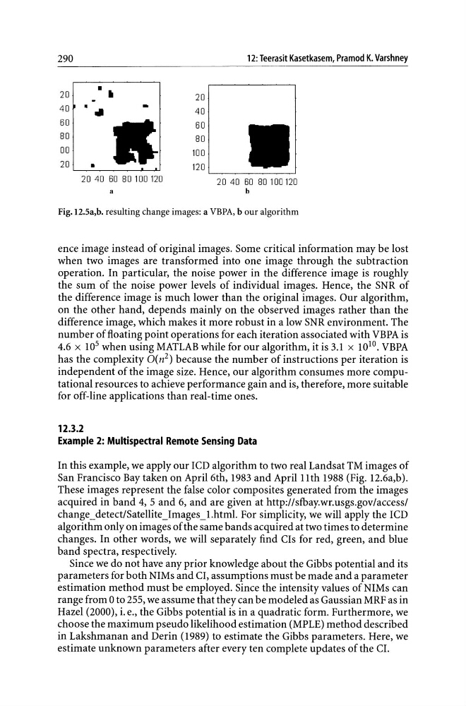
Fig.12.5a,b. resulting change images: a VBPA, b our algorithm
ence image instead of original images. Some critical information may be lost
when two images are transformed into one image through the subtraction
operation. In particular, the noise power in the difference image is roughly
the sum of the noise power levels of individual images. Hence, the SNR of
the difference image is much lower than the original images. Our algorithm,
on the other hand, depends mainly on the observed images rather than the
difference image, which makes it more robust in a low SNR environment. The
number of floating point operations for each iteration associated with VBPA is
4.6 x 10 5 when using MATLAB while for our algorithm, it is 3.1 x 10¹⁰. VBPA
has the complexity O(n 2 ) because the number of instructions per iteration is
independent of the image size. Hence, our algorithm consumes more computational resources to achieve performance gain and is, therefore, more suitable
for off-line applications than real-time ones.
12.3.2
Example 2: Multispectral Remote Sensing Data
In this example, we apply our ICD algorithm to two real Landsat TM images of
San Francisco Bay taken on April 6th, 1983 and April 11 th 1988 (Fig. 12.6a,b).
These images represent the false color composites generated from the images
acquired in band 4, 5 and 6, and are given at http://sfbay.wr.usgs.gov/access/
change_detect/Satellite_Images_1.html. For simplicity, we will apply the ICD
algorithm only on images of the same bands acquired at two times to determine
changes. In other words, we will separately find CIs for red, green, and blue
band spectra, respectively.
Since we do not have any prior knowledge about the Gibbs potential and its
parameters for both NIMs and CI, assumptions must be made and a parameter
estimation method must be employed. Since the intensity values of NIMs can
range from 0 to 255, we assume that they can be modeled as Gaussian MRF as in
Hazel (2000), i. e., the Gibbs potential is in a quadratic form. Furthermore, we
choose the maximum pseudo likelihood estimation (MPLE) method described
in Lakshmanan and Derin (1989) to estimate the Gibbs parameters. Here, we
estimate unknown parameters after every ten complete updates of the CI.
•
20
•
40
•
..
•
60
80
00
20
•
2040 60 80100120
a
20
40
60
80
100
12: Teerasit Kasetkasem, Pramod K. Varshney
120 L -_ _ _ _ _ ---'
2040 60 80100120
b
Fig.12.5a,b. resulting change images: a VBPA, b our algorithm
ence image instead of original images. Some critical information may be lost
when two images are transformed into one image through the subtraction
operation. In particular, the noise power in the difference image is roughly
the sum of the noise power levels of individual images. Hence, the SNR of
the difference image is much lower than the original images. Our algorithm,
on the other hand, depends mainly on the observed images rather than the
difference image, which makes it more robust in a low SNR environment. The
number of floating point operations for each iteration associated with VBPA is
4.6 x 10 5 when using MATLAB while for our algorithm, it is 3.1 x 10¹⁰. VBPA
has the complexity O(n 2 ) because the number of instructions per iteration is
independent of the image size. Hence, our algorithm consumes more computational resources to achieve performance gain and is, therefore, more suitable
for off-line applications than real-time ones.
12.3.2
Example 2: Multispectral Remote Sensing Data
In this example, we apply our ICD algorithm to two real Landsat TM images of
San Francisco Bay taken on April 6th, 1983 and April 11 th 1988 (Fig. 12.6a,b).
These images represent the false color composites generated from the images
acquired in band 4, 5 and 6, and are given at http://sfbay.wr.usgs.gov/access/
change_detect/Satellite_Images_1.html. For simplicity, we will apply the ICD
algorithm only on images of the same bands acquired at two times to determine
changes. In other words, we will separately find CIs for red, green, and blue
band spectra, respectively.
Since we do not have any prior knowledge about the Gibbs potential and its
parameters for both NIMs and CI, assumptions must be made and a parameter
estimation method must be employed. Since the intensity values of NIMs can
range from 0 to 255, we assume that they can be modeled as Gaussian MRF as in
Hazel (2000), i. e., the Gibbs potential is in a quadratic form. Furthermore, we
choose the maximum pseudo likelihood estimation (MPLE) method described
in Lakshmanan and Derin (1989) to estimate the Gibbs parameters. Here, we
estimate unknown parameters after every ten complete updates of the CI.