

252
10: Pakorn Watanachaturaporn, Manoj K. Arora
Polynomial Kernels of degrees 2 to 4
100
A-..I>..
...
90 ,~
ft
r
80
>./
fi
... 70
f!
I~
.7
~
60
...
~
... 50
"' l
40
~PoIyD2
• 30
-B-PoIyD3
5 2()
-fr-PoIy04
10
0
~' #" ~'
~,
~':, ,~ ,~ ,#' ,~ #"
~ .
~ .
~ .
' "
~ .
Penalty Value (C)
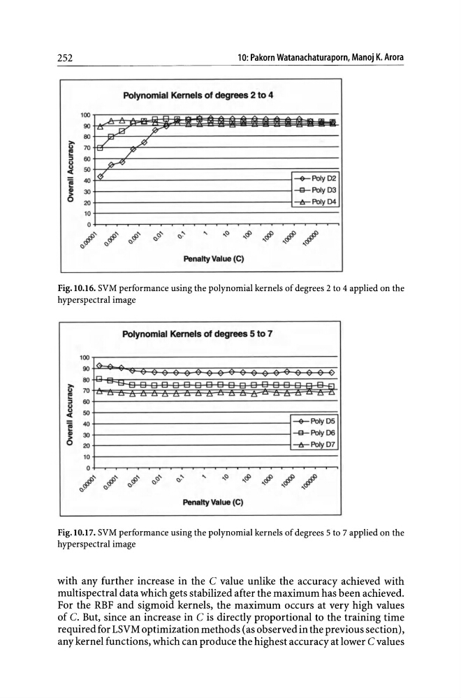
Fig. 10.16. SVM performance using the polynomial kernels of degrees 2 to 4 applied on the
hyperspectral image
Polynomial Kernels of degrees 5 t o 7
100
90
I~.L>.
1r::J
v
V'
V'
V'
V
V
v
80
=-.-.
, - , 0
>~
70
~<;>~
~~
~L.>
~~~
~u
L.>~
~
60
...
~ 50
f
40
~PoIyD5
5
30
-B-PoIyD6
2()
-fr-PoIyD7
10
0
~' #" ~'
~,
, , ,~ ,~ ,#' ,~ ,#"
~.
~ .
~ .
~ .
~ .
Penalty Value (C)
Fig. 10.17. SVM performance using the polynomial kernels of degrees 5 to 7 applied on the
hyperspectral image
with any further increase in the C value unlike the accuracy achieved with
multispectral data which gets stabilized after the maximum has been achieved.
For the RBF and sigmoid kernels, the maximum occurs at very high values
of C. But, since an increase in C is directly proportional to the training time
required for LSVM optimization methods (as observed in the previous section),
any kernel functions , which can produce the highest accuracy at lower C values
10: Pakorn Watanachaturaporn, Manoj K. Arora
Polynomial Kernels of degrees 2 to 4
100
A-..I>..
...
90 ,~
ft
r
80
>./
fi
... 70
f!
I~
.7
~
60
...
~
... 50
"' l
40
~PoIyD2
• 30
-B-PoIyD3
5 2()
-fr-PoIy04
10
0
~' #" ~'
~,
~':, ,~ ,~ ,#' ,~ #"
~ .
~ .
~ .
' "
~ .
Penalty Value (C)
Fig. 10.16. SVM performance using the polynomial kernels of degrees 2 to 4 applied on the
hyperspectral image
Polynomial Kernels of degrees 5 t o 7
100
90
I~.L>.
1r::J
v
V'
V'
V'
V
V
v
80
=-.-.
, - , 0
>~
70
~<;>~
~~
~L.>
~~~
~u
L.>~
~
60
...
~ 50
f
40
~PoIyD5
5
30
-B-PoIyD6
2()
-fr-PoIyD7
10
0
~' #" ~'
~,
, , ,~ ,~ ,#' ,~ ,#"
~.
~ .
~ .
~ .
~ .
Penalty Value (C)
Fig. 10.17. SVM performance using the polynomial kernels of degrees 5 to 7 applied on the
hyperspectral image
with any further increase in the C value unlike the accuracy achieved with
multispectral data which gets stabilized after the maximum has been achieved.
For the RBF and sigmoid kernels, the maximum occurs at very high values
of C. But, since an increase in C is directly proportional to the training time
required for LSVM optimization methods (as observed in the previous section),
any kernel functions , which can produce the highest accuracy at lower C values