

Hyperspectral Classification Using ICA Based Mixture Model
221
2. Randomly initialize the mixing matrix Aj and the bias vector bj, for each
class j, where j = 1 to K.
For t = 1 to T do
Step 2: Estimate the vector of independent components Sj,t as given in (9.4).
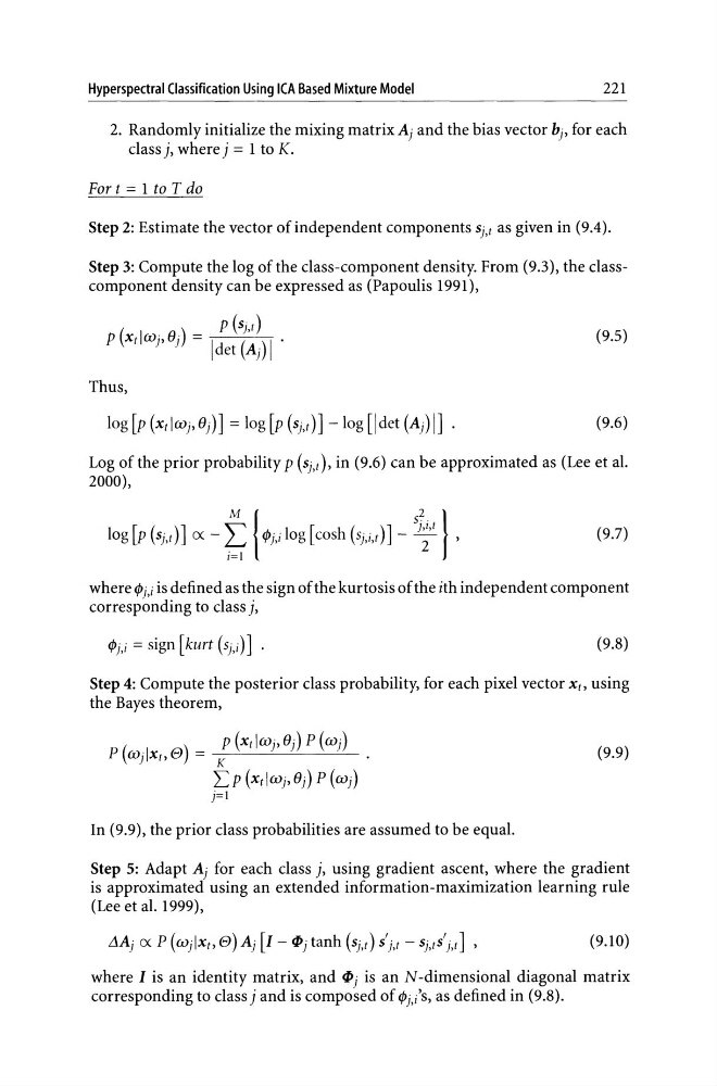
Step 3: Compute the log of the class-component density. From (9.3), the classcomponent density can be expressed as (Papoulis 1991),
(9.5)
Thus,
(9.6)
Log of the prior probability p (Sj,t), in (9.6) can be approximated as (Lee et al.
2000),
M I
52.\
log [p (Sj,t)] ex - ~ tPj,dog [cosh (Sj,i,t)] _ J~,t ,
(9.7)
where tPj,i is defined as the sign of the kurtosis of the ith independent component
corresponding to class j,
tPj,i = sign [kurt (Sj,i)] •
(9.8)
Step 4: Compute the posterior class probability, for each pixel vector Xt> using
the Bayes theorem,
(
)
P (Xtlcuj,8j) P (Wj)
P Wj IXt> e = --=K,,------'----'-----'-'--..:........:-'-LP (xtl wj,8j) P (Wj)
j=l
In (9.9), the prior class probabilities are assumed to be equal.
(9.9)
Step 5: Adapt Aj for each class j, using gradient ascent, where the gradient
is approximated using an extended information-maximization learning rule
(Lee et al. 1999),
(9.10)
where I is an identity matrix, and q,j is an N-dimensional diagonal matrix
corresponding to class j and is composed of tPj,i's, as defined in (9.8).
221
2. Randomly initialize the mixing matrix Aj and the bias vector bj, for each
class j, where j = 1 to K.
For t = 1 to T do
Step 2: Estimate the vector of independent components Sj,t as given in (9.4).
Step 3: Compute the log of the class-component density. From (9.3), the classcomponent density can be expressed as (Papoulis 1991),
(9.5)
Thus,
(9.6)
Log of the prior probability p (Sj,t), in (9.6) can be approximated as (Lee et al.
2000),
M I
52.\
log [p (Sj,t)] ex - ~ tPj,dog [cosh (Sj,i,t)] _ J~,t ,
(9.7)
where tPj,i is defined as the sign of the kurtosis of the ith independent component
corresponding to class j,
tPj,i = sign [kurt (Sj,i)] •
(9.8)
Step 4: Compute the posterior class probability, for each pixel vector Xt> using
the Bayes theorem,
(
)
P (Xtlcuj,8j) P (Wj)
P Wj IXt> e = --=K,,------'----'-----'-'--..:........:-'-LP (xtl wj,8j) P (Wj)
j=l
In (9.9), the prior class probabilities are assumed to be equal.
(9.9)
Step 5: Adapt Aj for each class j, using gradient ascent, where the gradient
is approximated using an extended information-maximization learning rule
(Lee et al. 1999),
(9.10)
where I is an identity matrix, and q,j is an N-dimensional diagonal matrix
corresponding to class j and is composed of tPj,i's, as defined in (9.8).