Markov Random Field Models
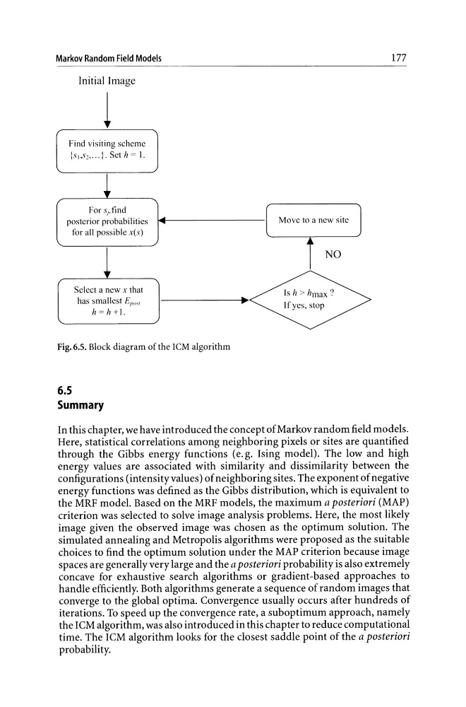
Initial Image
1
Find visiting scheme
{SJ,S2""}' Set h = 1.
For sj> find
posterior probabilities
for all possible x(s)
Select a new x that
has smallest £1'0."
h=h+1.
Fig.6.5. Block diagram of the I eM algorithm
6.5
Summary
Move to a new site
NO
Is h > hmax ?
If yes, stop
177
In this chapter, we have introduced the concept of Markov random field models.
Here, statistical correlations among neighboring pixels or sites are quantified
through the Gibbs energy functions (e. g. Ising model). The low and high
energy values are associated with similarity and dissimilarity between the
configurations (intensity values ) of neighboring sites. The exponent of negative
energy functions was defined as the Gibbs distribution, which is equivalent to
the MRF model. Based on the MRF models, the maximum a posteriori (MAP)
criterion was selected to solve image analysis problems. Here, the most likely
image given the observed image was chosen as the optimum solution. The
simulated annealing and Metropolis algorithms were proposed as the suitable
choices to find the optimum solution under the MAP criterion because image
spaces are generally very large and the a posteriori probability is also extremely
concave for exhaustive search algorithms or gradient-based approaches to
handle efficiently. Both algorithms generate a sequence of random images that
converge to the global optima. Convergence usually occurs after hundreds of
iterations. To speed up the convergence rate, a suboptimum approach, namely
the ICM algorithm, was also introduced in this chapter to reduce computational
time. The ICM algorithm looks for the closest saddle point of the a posteriori
probability.