

Support Vector Machines
145
From the point of view of statistical learning theory, it can be shown that the
minimization of the VC-dimension is achieved by minimizing the first term
of (5.32) similar to the linearly separable case. Unlike the linearly separable
case, minimization of the empirical risk in this case is achieved by minimizing
the second term of (5.32). Thus, here also, the principle of structural risk
minimization is satisfied.
The constrained optimization problem given by (5.32) to (5.34) is again
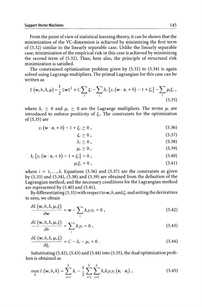
solved using Lagrange multipliers. The primal Lagrangian for this case can be
written as
(5.35)
where Ai ::: 0 and Pi ::: 0 are the Lagrange multipliers. The terms Pi are
introduced to enforce positivity of ~i. The constraints for the optimization
of (5.35) are
y;( w . Xi + b) - 1 + ~i ::: 0 ,
~i ::: 0 ,
Ai ::: 0 ,
Pi ::: 0 ,
A;/Yi (w. Xi + b) - 1 +~;} = 0 ,
Pi~i = 0,
(5.36)
(5.37)
(5.38)
(5.39)
(5.40)
(5.41)
where i = 1, ... , k. Equations (5.36) and (5.37) are the constraints as given
by (5.33) and (5.34), (5.38) and (5.39) are obtained from the definition of the
Lagrangian method, and the necessary conditions for the Lagrangian method
are represented by (5.40) and (5.41).
By differentiating (5.35) with respect to w, b, and ~i and setting the derivatives
to zero, we obtain
aL(w,b,A,p,~) -w- "1 y . X .-0
a
-
~/I.11 1 -
,
W
.
1
aL (w, b,A,p,~) = " ky. = 0
ab
~ 11
,
1
aL (w, b,A, p,~)
--'-------'- = C -Ai - Pi = o.
a~i
(5.42)
(5.43)
(5.44)
Substituting (5.42), (5.43) and (5.44) into (5.35), the dual optimization problem is obtained as
k
1 k k
mlxL (w, b,A) = LAi - 2: L LAiAjYiYj (Xi· Xj) ,
1=1
1=1 7=1
(5.45)
145
From the point of view of statistical learning theory, it can be shown that the
minimization of the VC-dimension is achieved by minimizing the first term
of (5.32) similar to the linearly separable case. Unlike the linearly separable
case, minimization of the empirical risk in this case is achieved by minimizing
the second term of (5.32). Thus, here also, the principle of structural risk
minimization is satisfied.
The constrained optimization problem given by (5.32) to (5.34) is again
solved using Lagrange multipliers. The primal Lagrangian for this case can be
written as
(5.35)
where Ai ::: 0 and Pi ::: 0 are the Lagrange multipliers. The terms Pi are
introduced to enforce positivity of ~i. The constraints for the optimization
of (5.35) are
y;( w . Xi + b) - 1 + ~i ::: 0 ,
~i ::: 0 ,
Ai ::: 0 ,
Pi ::: 0 ,
A;/Yi (w. Xi + b) - 1 +~;} = 0 ,
Pi~i = 0,
(5.36)
(5.37)
(5.38)
(5.39)
(5.40)
(5.41)
where i = 1, ... , k. Equations (5.36) and (5.37) are the constraints as given
by (5.33) and (5.34), (5.38) and (5.39) are obtained from the definition of the
Lagrangian method, and the necessary conditions for the Lagrangian method
are represented by (5.40) and (5.41).
By differentiating (5.35) with respect to w, b, and ~i and setting the derivatives
to zero, we obtain
aL(w,b,A,p,~) -w- "1 y . X .-0
a
-
~/I.11 1 -
,
W
.
1
aL (w, b,A,p,~) = " ky. = 0
ab
~ 11
,
1
aL (w, b,A, p,~)
--'-------'- = C -Ai - Pi = o.
a~i
(5.42)
(5.43)
(5.44)
Substituting (5.42), (5.43) and (5.44) into (5.35), the dual optimization problem is obtained as
k
1 k k
mlxL (w, b,A) = LAi - 2: L LAiAjYiYj (Xi· Xj) ,
1=1
1=1 7=1
(5.45)