

122
4: Stefan A. Robila
To find the independent components, we proceed to determine the projection vector WI such that wi x is as non-Gaussian as possible. We then search
for a second projection vector W2 such that wi x is as non-Gaussian as possible, making sure that the projection is orthogonal to the one already found.
The process continues until all the projection vectors (WI. W2, W3, ... , wm ) are
found. It can be shown (Hyvarinen et al. 2001) that, if we consider:
u=Wx=WAs,
(4.43)
where W = (WI. W2, W3,"" wm)T, the components of u are estimates of the
original independent components (s).
There are several methods for quantifying the non-Gaussianity. One of them
is based on the negentropy, (i. e. the distance between the probability density
function of the component and the Gaussian probability density function)
(Common 1994). For a random vector u the negentropy is defined as:
J(u) = H (uG) - H(u) ,
( 4.44)
where UG denotes a Gaussian variable with the same covariance as u.
While negentropy is a good measure for non-Gaussianity, it is difficult to use
it in practice due to the need for an accurate approximation for the probability
density function. Instead, approximations of the entropy have been suggested.
One approximation is based on general nonquadratic functions and the other
one is based on skewness and kurtosis. In both cases, once the approximate
formula for negentropy is computed a gradient-based algorithm is devised.
In the first case, the negentropy for a random variable u is approximated as
(Hyvarinen et al. 2001):
J(u) = [E{G(u)} -E{G(UG)}]2 ,
(4.45)
where G(·) is a general nonquadratic function. It is interesting to note that
again, as in the case of information maximization, the accuracy of the results
relies heavily on the choice of the function. Additionally, in this case, the
independent components are sequentially generated, making sure that they
remain uncorrelated.
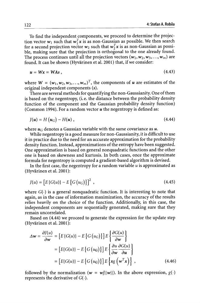
Based on (4.44) we proceed to generate the expression for the update step
(Hyvarinen et al. 2001):
Llw = -
= [E{G(u)} - E {G (uG)}] E -
oJ(u)
{OG(U) }
ow
ow
{
ou OG(U)}
= [E{G(u)}-E{G(uG)}]E - - -
ow ou
= [E{G(U)}-E{G(UG)}]E{xg(wTx)} ,
( 4.46)
followed by the normalization (w = w/llwll). In the above expression, g(-)
represents the derivative of G(·).
4: Stefan A. Robila
To find the independent components, we proceed to determine the projection vector WI such that wi x is as non-Gaussian as possible. We then search
for a second projection vector W2 such that wi x is as non-Gaussian as possible, making sure that the projection is orthogonal to the one already found.
The process continues until all the projection vectors (WI. W2, W3, ... , wm ) are
found. It can be shown (Hyvarinen et al. 2001) that, if we consider:
u=Wx=WAs,
(4.43)
where W = (WI. W2, W3,"" wm)T, the components of u are estimates of the
original independent components (s).
There are several methods for quantifying the non-Gaussianity. One of them
is based on the negentropy, (i. e. the distance between the probability density
function of the component and the Gaussian probability density function)
(Common 1994). For a random vector u the negentropy is defined as:
J(u) = H (uG) - H(u) ,
( 4.44)
where UG denotes a Gaussian variable with the same covariance as u.
While negentropy is a good measure for non-Gaussianity, it is difficult to use
it in practice due to the need for an accurate approximation for the probability
density function. Instead, approximations of the entropy have been suggested.
One approximation is based on general nonquadratic functions and the other
one is based on skewness and kurtosis. In both cases, once the approximate
formula for negentropy is computed a gradient-based algorithm is devised.
In the first case, the negentropy for a random variable u is approximated as
(Hyvarinen et al. 2001):
J(u) = [E{G(u)} -E{G(UG)}]2 ,
(4.45)
where G(·) is a general nonquadratic function. It is interesting to note that
again, as in the case of information maximization, the accuracy of the results
relies heavily on the choice of the function. Additionally, in this case, the
independent components are sequentially generated, making sure that they
remain uncorrelated.
Based on (4.44) we proceed to generate the expression for the update step
(Hyvarinen et al. 2001):
Llw = -
= [E{G(u)} - E {G (uG)}] E -
oJ(u)
{OG(U) }
ow
ow
{
ou OG(U)}
= [E{G(u)}-E{G(uG)}]E - - -
ow ou
= [E{G(U)}-E{G(UG)}]E{xg(wTx)} ,
( 4.46)
followed by the normalization (w = w/llwll). In the above expression, g(-)
represents the derivative of G(·).