

Independent Component Analysis
III
solution consists of the unique independent non-Gaussian components and
of mixtures of independent Gaussian components (Hyvarinen et al. 2001).
However, when only one of the components is Gaussian, the ICA solution in
terms of independent components can still be correctly obtained. Since in
many signal and image processing applications, the noise is considered to
be Gaussian, relaxing restriction i) to include a Gaussian component allows
greater applicability of ICA.
A very simple method for selecting the non-Gaussian variables is based
on kurtosis. Kurtosis is the fourth order central moment and, for a random
variable u, is defined in the normalized form as (Common 1994):
(4.3)
In general, for a random variable u, E {j(u)} denotes the expected value of
f(u) where f(·) is a function of u. With this notation, E{ u} is the expected value
of u (or average of u for the discrete case).
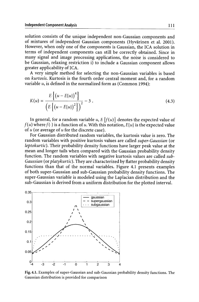
For Gaussian distributed random variables, the kurtosis value is zero. The
random variables with positive kurtosis values are called super-Gaussian (or
leptokurtic). Their probability density functions have larger peak value at the
mean and longer tails when compared with the Gaussian probability density
function. The random variables with negative kurtosis values are called subGaussian (or platykurtic). They are characterized by flatter probability density
functions than that of the normal variables. Figure 4.1 presents examples
of both super-Gaussian and sub-Gaussian probability density functions. The
super-Gaussian variable is modeled using the Laplacian distribution and the
sub-Gaussian is derived from a uniform distribution for the plotted interval.
0.35
0.3
0.25
0.2
0.15
0.1
0.05
0
·4
-··~·-T~-~-~-~~-··
./
....
...
·3
·2
I
I
·1
/1
/ ,
0
-
gaussian
- - supergaussian
. . . subgaussian
\
, , ,
" ....
2
3
4
Fig.4.1. Examples of super-Gaussian and sub-Gaussian probability density functions. The
Gaussian distribution is provided for comparison
III
solution consists of the unique independent non-Gaussian components and
of mixtures of independent Gaussian components (Hyvarinen et al. 2001).
However, when only one of the components is Gaussian, the ICA solution in
terms of independent components can still be correctly obtained. Since in
many signal and image processing applications, the noise is considered to
be Gaussian, relaxing restriction i) to include a Gaussian component allows
greater applicability of ICA.
A very simple method for selecting the non-Gaussian variables is based
on kurtosis. Kurtosis is the fourth order central moment and, for a random
variable u, is defined in the normalized form as (Common 1994):
(4.3)
In general, for a random variable u, E {j(u)} denotes the expected value of
f(u) where f(·) is a function of u. With this notation, E{ u} is the expected value
of u (or average of u for the discrete case).
For Gaussian distributed random variables, the kurtosis value is zero. The
random variables with positive kurtosis values are called super-Gaussian (or
leptokurtic). Their probability density functions have larger peak value at the
mean and longer tails when compared with the Gaussian probability density
function. The random variables with negative kurtosis values are called subGaussian (or platykurtic). They are characterized by flatter probability density
functions than that of the normal variables. Figure 4.1 presents examples
of both super-Gaussian and sub-Gaussian probability density functions. The
super-Gaussian variable is modeled using the Laplacian distribution and the
sub-Gaussian is derived from a uniform distribution for the plotted interval.
0.35
0.3
0.25
0.2
0.15
0.1
0.05
0
·4
-··~·-T~-~-~-~~-··
./
....
...
·3
·2
I
I
·1
/1
/ ,
0
-
gaussian
- - supergaussian
. . . subgaussian
\
, , ,
" ....
2
3
4
Fig.4.1. Examples of super-Gaussian and sub-Gaussian probability density functions. The
Gaussian distribution is provided for comparison