

2.9 SKY RADIANCE
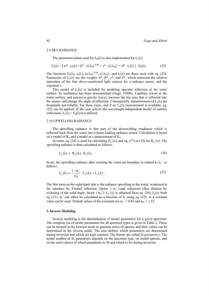
The parameterization used for E d (Ȝ) is also implemented for L s (Ȝ):
L s (Ȝ) = [ Į* · t A (Ȝ) + ȕ* · (Ȝ/Ȝ R )
-4.09 + Ȗ* · (Ȝ/Ȝ M )
v + į* · t C (Ȝ) ] · E 0 (Ȝ).
(25)
The functions E 0 (Ȝ), t A (Ȝ), (Ȝ/Ȝ R )
-4.09 , (Ȝ/Ȝ M )
v , and t C (Ȝ) are those used with eq. (23).
Parameters of L s (Ȝ) are the weights Į*, ȕ*, Ȗ*, and į*, which represent the relative
intensities of the four above-mentioned light sources for a radiance sensor, and the
exponent v.
This model of L s (Ȝ) is included for modeling specular reflection at the water
surface. Its usefulness has been demonstrated (Gege, 1998b). Capillary waves at the
water surface, and moreover gravity waves, increase the sky area that is reflected into
the sensor, and change the angle of reflection. Consequently, measurements of L s (Ȝ) are
frequently not reliable. For these cases, and if no L s (Ȝ) measurement is available, eq.
(25) can be applied. If the user selects the wavelength-independent model of surface
reflections, L s (Ȝ) = E d (Ȝ)/ʌ is utilized.
2.10 UPWELLING RADIANCE
The upwelling radiance is that part of the downwelling irradiance which is
reflected back from the water into a down-looking radiance sensor. Calculation is based
on a model of R rs and a model or a measurement of E d .
In water, eq. (24) is used for calculating E d
− (Ȝ), and eq. (17) or (19) for R rs
− (Ȝ). The
upwelling radiance is then calculated as follows:
.
)
(
E
)
(
R
)
(
L
d
rs
u
λ
⋅
λ
=
λ
−
−
−
(26)
In air, the upwelling radiance after crossing the water-air boundary is related to L u
− as
follows:
.
)
(
L
)
(
L
n
1
)
(
L
r
u
2
W
L
u
λ
+
λ
⋅
σ
−
=
λ
−
−
(27)
The first term on the right-hand side is the radiance upwelling in the water, weakened at
the interface by Fresnel reflection (factor 1–ı L
− ) and refraction (flux dilution by
widening of the solid angle, factor 1/n w
2 ). L u
− (Ȝ) is obtained from eq. (26), L r (Ȝ) from
eq. (11). ı L
− can either be calculated as a function of ș v using eq. (12), or a constant
value can be used. Default values of the constants are ı L
− = 0.02 and n W = 1.33.
3. Inverse Modeling
Inverse modeling is the determination of model parameters for a given spectrum.
The complete list of model parameters for all spectrum types is given in Table 2. These
can be iterated in the forward mode to generate series of spectra, and their values can be
determined in the inverse mode. The user defines which parameters are determined
during inversion and which are kept constant. The former are called fit parameters. The
actual number of fit parameters depends on the spectrum type, on model options, and
on the user's choice of which parameters to fit and which to fix during inversion.
92
Gege and Albert
The parameterization used for E d (Ȝ) is also implemented for L s (Ȝ):
L s (Ȝ) = [ Į* · t A (Ȝ) + ȕ* · (Ȝ/Ȝ R )
-4.09 + Ȗ* · (Ȝ/Ȝ M )
v + į* · t C (Ȝ) ] · E 0 (Ȝ).
(25)
The functions E 0 (Ȝ), t A (Ȝ), (Ȝ/Ȝ R )
-4.09 , (Ȝ/Ȝ M )
v , and t C (Ȝ) are those used with eq. (23).
Parameters of L s (Ȝ) are the weights Į*, ȕ*, Ȗ*, and į*, which represent the relative
intensities of the four above-mentioned light sources for a radiance sensor, and the
exponent v.
This model of L s (Ȝ) is included for modeling specular reflection at the water
surface. Its usefulness has been demonstrated (Gege, 1998b). Capillary waves at the
water surface, and moreover gravity waves, increase the sky area that is reflected into
the sensor, and change the angle of reflection. Consequently, measurements of L s (Ȝ) are
frequently not reliable. For these cases, and if no L s (Ȝ) measurement is available, eq.
(25) can be applied. If the user selects the wavelength-independent model of surface
reflections, L s (Ȝ) = E d (Ȝ)/ʌ is utilized.
2.10 UPWELLING RADIANCE
The upwelling radiance is that part of the downwelling irradiance which is
reflected back from the water into a down-looking radiance sensor. Calculation is based
on a model of R rs and a model or a measurement of E d .
In water, eq. (24) is used for calculating E d
− (Ȝ), and eq. (17) or (19) for R rs
− (Ȝ). The
upwelling radiance is then calculated as follows:
.
)
(
E
)
(
R
)
(
L
d
rs
u
λ
⋅
λ
=
λ
−
−
−
(26)
In air, the upwelling radiance after crossing the water-air boundary is related to L u
− as
follows:
.
)
(
L
)
(
L
n
1
)
(
L
r
u
2
W
L
u
λ
+
λ
⋅
σ
−
=
λ
−
−
(27)
The first term on the right-hand side is the radiance upwelling in the water, weakened at
the interface by Fresnel reflection (factor 1–ı L
− ) and refraction (flux dilution by
widening of the solid angle, factor 1/n w
2 ). L u
− (Ȝ) is obtained from eq. (26), L r (Ȝ) from
eq. (11). ı L
− can either be calculated as a function of ș v using eq. (12), or a constant
value can be used. Default values of the constants are ı L
− = 0.02 and n W = 1.33.
3. Inverse Modeling
Inverse modeling is the determination of model parameters for a given spectrum.
The complete list of model parameters for all spectrum types is given in Table 2. These
can be iterated in the forward mode to generate series of spectra, and their values can be
determined in the inverse mode. The user defines which parameters are determined
during inversion and which are kept constant. The former are called fit parameters. The
actual number of fit parameters depends on the spectrum type, on model options, and
on the user's choice of which parameters to fit and which to fix during inversion.
92
Gege and Albert