

2006). These approaches need refinement with more field data to account for the
optical variability of all OSCs, and they also need regional tuning for the different
mixtures of OSCs found in coastal waters. In particular, there has been the lack of
a general approach to remove the bottom signal in optically shallow waters
(Cannizzaro and Carder 2006), and, in particular, this problem needs to be
addressed around coral reefs.
One difficulty in the past has been the lack of reliable in situ Chl data with
sufficient spatial and temporal coverage to validate satellite Chl under all possible
circumstances. Despite more than a decade of SIMBIOS effort, most ocean waters
are still under-sampled. This lack of data inherently hinders any effort for algorithm coefficient tuning of both empirical and semi-analytical algorithms. Systematic measurements of Chl using autonomous platforms such as gliders, drifters,
or marine buoys, may help overcome this difficulty and eventually lead to
improved algorithms and better data products.
The benefits of ocean color measurements extend beyond Chl. Recent efforts
have used multi-band R rs or optical models to classify major phytoplankton
functional types (PFTs) in the global ocean (Subramaniam et al. 1999; Alvain et al.
2005; Westberry and Siegel 2006; Nair et al. 2008; Mouw and Yoder 2010). This
is possible, in theory at least, because different PFTs have different pigment
composition, resulting in distinguishable pigment absorption and R rs spectral
shapes. On regional scales, Sathyendranath et al. (2004) developed an optical
inversion model to separate diatom blooms from other blooms in the North
Atlantic. Cannizzaro et al. (2008) used backscattering/Chl ratios (or backscattering
efficiency) and Tomlinson et al. (2009) used R rs spectral curvatures in the bluegreen to distinguish K. brevis blooms from other blooms on the West Florida
Shelf. Further efforts are required to characterize the optical properties (absorption
Jan03 Jan04 Jan05 Jan06 Jan07 Jan08 Jan09 Jan10
MODISA/SeaWiFS Chl ratio
0.8
0.9
1.0
1.1
1.2
% coverage
0
20
40
60
80
100
OCx
CI
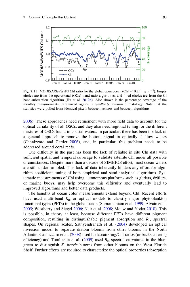
Fig. 7.11 MODISA/SeaWiFS Chl ratio for the global open ocean (Chl B 0.25 mg m
-3
). Empty
circles are from the operational (OCx) band-ratio algorithms, and filled circles are from the CI
band-subtraction algorithm (Hu et al. 2012b). Also shown is the percentage coverage of the
monthly measurements, referenced against a SeaWiFS mission climatology. Note that the
statistics were pulled from identical pixels between sensors and between algorithms
7 Oceanic Chlorophyll-a Content
193
optical variability of all OSCs, and they also need regional tuning for the different
mixtures of OSCs found in coastal waters. In particular, there has been the lack of
a general approach to remove the bottom signal in optically shallow waters
(Cannizzaro and Carder 2006), and, in particular, this problem needs to be
addressed around coral reefs.
One difficulty in the past has been the lack of reliable in situ Chl data with
sufficient spatial and temporal coverage to validate satellite Chl under all possible
circumstances. Despite more than a decade of SIMBIOS effort, most ocean waters
are still under-sampled. This lack of data inherently hinders any effort for algorithm coefficient tuning of both empirical and semi-analytical algorithms. Systematic measurements of Chl using autonomous platforms such as gliders, drifters,
or marine buoys, may help overcome this difficulty and eventually lead to
improved algorithms and better data products.
The benefits of ocean color measurements extend beyond Chl. Recent efforts
have used multi-band R rs or optical models to classify major phytoplankton
functional types (PFTs) in the global ocean (Subramaniam et al. 1999; Alvain et al.
2005; Westberry and Siegel 2006; Nair et al. 2008; Mouw and Yoder 2010). This
is possible, in theory at least, because different PFTs have different pigment
composition, resulting in distinguishable pigment absorption and R rs spectral
shapes. On regional scales, Sathyendranath et al. (2004) developed an optical
inversion model to separate diatom blooms from other blooms in the North
Atlantic. Cannizzaro et al. (2008) used backscattering/Chl ratios (or backscattering
efficiency) and Tomlinson et al. (2009) used R rs spectral curvatures in the bluegreen to distinguish K. brevis blooms from other blooms on the West Florida
Shelf. Further efforts are required to characterize the optical properties (absorption
Jan03 Jan04 Jan05 Jan06 Jan07 Jan08 Jan09 Jan10
MODISA/SeaWiFS Chl ratio
0.8
0.9
1.0
1.1
1.2
% coverage
0
20
40
60
80
100
OCx
CI
Fig. 7.11 MODISA/SeaWiFS Chl ratio for the global open ocean (Chl B 0.25 mg m
-3
). Empty
circles are from the operational (OCx) band-ratio algorithms, and filled circles are from the CI
band-subtraction algorithm (Hu et al. 2012b). Also shown is the percentage coverage of the
monthly measurements, referenced against a SeaWiFS mission climatology. Note that the
statistics were pulled from identical pixels between sensors and between algorithms
7 Oceanic Chlorophyll-a Content
193