

Surface current maps Routine observations of surface currents are carried out in
the southern section of the Great Barrier Reef under the Australian Integrated
Marine Observing System (IMOS) using a phased-array HF radar system. Figure 13.2 shows an unsmoothed 10-minute sample of the surface currents. The spatial
structure captured in this map shows convergence zones, eddies, and jets on a scale
suitable for understanding the dynamics of the ocean between and around reefs.
Lagrangian tracking and connectivity Data like those shown in Fig. 13.2 can
be improved through a quality control evaluation of the data points themselves.
Mantovanelli et al. (2010) accomplished this by first removing the tidal variation at
each grid point, and then applying outlier removal techniques to the residuals on
the 10 min data. They then reinstated the tidal signal to calculate good quality
hourly averages of currents that can be used for Lagrangian tracking. This is a
mathematical procedure that uses spatial maps of surface current data taken at
successive time steps to produce tracks of buoyant particles. Lagrangian tracking
from HF ocean radar in the southern Great Barrier Reef is now sufficiently
accurate and robust to be able to investigate details of connectivity between coral
reefs. These are useful in conjunction with species behavior models for tracking
larvae, and in the movement of nutrients. Lagrangian tracking is also a useful
technique for search-and-rescue (Ullman et al. 2006) and for pollution management. The example shown in Fig. 13.5 is the result of a simultaneous release of an
instrumented drifter and the commencement of a Lagrangian track on the HF
radar.
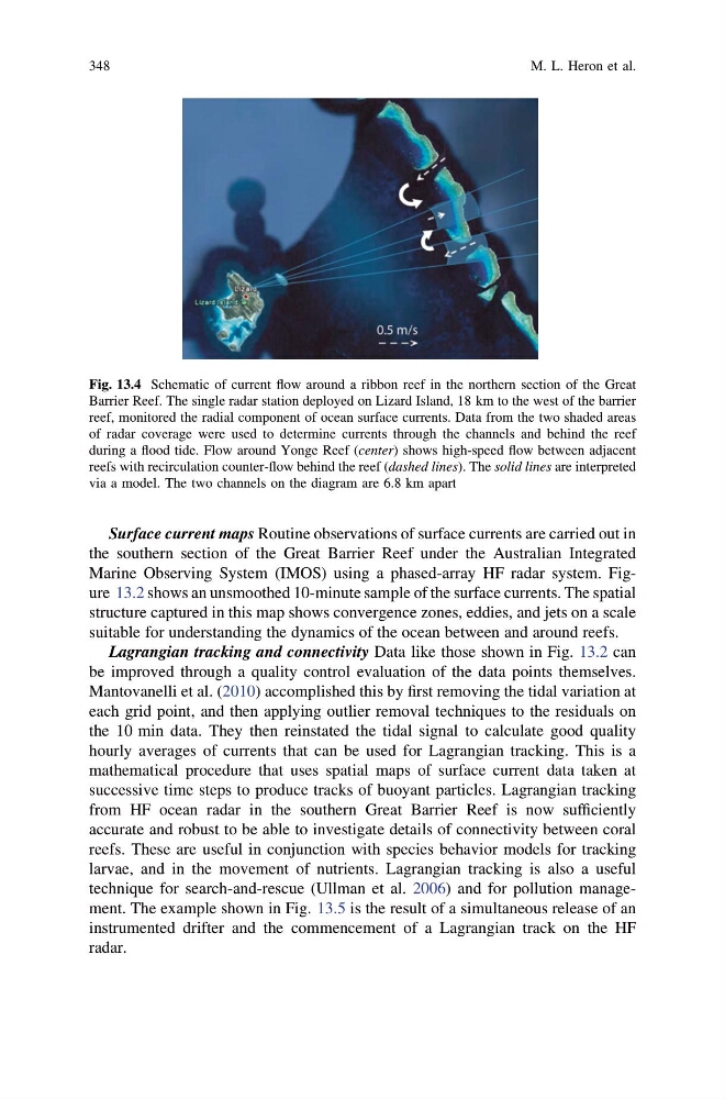
Fig. 13.4 Schematic of current flow around a ribbon reef in the northern section of the Great
Barrier Reef. The single radar station deployed on Lizard Island, 18 km to the west of the barrier
reef, monitored the radial component of ocean surface currents. Data from the two shaded areas
of radar coverage were used to determine currents through the channels and behind the reef
during a flood tide. Flow around Yonge Reef (center) shows high-speed flow between adjacent
reefs with recirculation counter-flow behind the reef (dashed lines). The solid lines are interpreted
via a model. The two channels on the diagram are 6.8 km apart
348
M. L. Heron et al.
the southern section of the Great Barrier Reef under the Australian Integrated
Marine Observing System (IMOS) using a phased-array HF radar system. Figure 13.2 shows an unsmoothed 10-minute sample of the surface currents. The spatial
structure captured in this map shows convergence zones, eddies, and jets on a scale
suitable for understanding the dynamics of the ocean between and around reefs.
Lagrangian tracking and connectivity Data like those shown in Fig. 13.2 can
be improved through a quality control evaluation of the data points themselves.
Mantovanelli et al. (2010) accomplished this by first removing the tidal variation at
each grid point, and then applying outlier removal techniques to the residuals on
the 10 min data. They then reinstated the tidal signal to calculate good quality
hourly averages of currents that can be used for Lagrangian tracking. This is a
mathematical procedure that uses spatial maps of surface current data taken at
successive time steps to produce tracks of buoyant particles. Lagrangian tracking
from HF ocean radar in the southern Great Barrier Reef is now sufficiently
accurate and robust to be able to investigate details of connectivity between coral
reefs. These are useful in conjunction with species behavior models for tracking
larvae, and in the movement of nutrients. Lagrangian tracking is also a useful
technique for search-and-rescue (Ullman et al. 2006) and for pollution management. The example shown in Fig. 13.5 is the result of a simultaneous release of an
instrumented drifter and the commencement of a Lagrangian track on the HF
radar.
Fig. 13.4 Schematic of current flow around a ribbon reef in the northern section of the Great
Barrier Reef. The single radar station deployed on Lizard Island, 18 km to the west of the barrier
reef, monitored the radial component of ocean surface currents. Data from the two shaded areas
of radar coverage were used to determine currents through the channels and behind the reef
during a flood tide. Flow around Yonge Reef (center) shows high-speed flow between adjacent
reefs with recirculation counter-flow behind the reef (dashed lines). The solid lines are interpreted
via a model. The two channels on the diagram are 6.8 km apart
348
M. L. Heron et al.