

width, but at a spatial resolution of 300 m. At the other end of the design spectrum
the Ikonos sensor provides 4 m pixels but at lower radiometric accuracy and in
only four spectral bands of 65–100 nm width. This design trade-off represents a
data level decision for the application of coral reef remote sensing methods. The
research indicates that all factors should be optimized, in that coral reef applications benefit from high spatial resolution, high spectral resolution and high
radiometric accuracy (Caplosini et al. 2003; Mumby et al. 1997; Mumby and
Edwards 2002). However, all three factors cannot be simultaneously maximized,
so in practice there must always be a trade-off when choosing a data source for a
given application. Note also that bands in the near and far infrared are largely
unusable for sub-surface mapping as water is practically opaque in wavelengths
above 700 nm (Fig. 4.2). Therefore, although an instrument such as Hyperion has
224 bands, only around 30 carry sufficient information for sub-surface
applications.
Airborne sensors are the ‘exception that proves the rule’ of the above described
sensor-design constraint since they fly closer to the Earth’s surface. A smaller
pixel therefore appears equivalent to a larger one in the sensor field of view, and it
is possible to achieve relatively high spatial and spectral resolution simultaneously. However, airborne data introduces numerous processing challenges.
Airborne hyperspectral sensors typically operate in a ‘push-broom’ design, where
the sensor records a line of pixels moved across the water surface by the forward
motion of the plane. The roll and yaw of the plane must be minimized in flight but
still require specialized image geo-correction. Closer proximity to the water surface introduces ‘cross track’ variation, where the view angle is different onto the
water surface to the left and the right of the aircraft travel. Careful flight line
design can minimize this (discussed later) but special image corrections are generally required. In all cases the quality of airborne imagery can be substantially
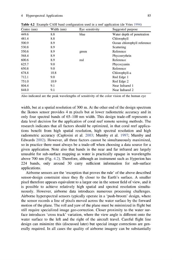
Table 4.2 Example CASI band configuration used in a reef application (de Vries 1994)
Centre (nm)
Width (nm)
Eye sensitivity
Suggested purpose
449.6
8.8
blue
Water depth of penetration
481.4
8.8
Chlorophyll
500.9
8.9
Ocean chlorophyll reference
530.8
8.9
Scattering
550.6
8.9
green
Reference
568.4
8.9
Phycoerythrin
600.6
8.9
red
Reference
625.7
9.0
Phycocyanin
650.8
9.0
Reference
678.8
10.8
Chlorophyll-a
712.1
9.0
Red Edge 1
751.0
10.9
Red Edge 2
804.4
9.1
Near Infrared 1
848.0
9.1
Near Infrared 2
Also indicated are the peak wavelengths of sensitivity of the color vision of the human eye
4 Hyperspectral Applications
85
the Ikonos sensor provides 4 m pixels but at lower radiometric accuracy and in
only four spectral bands of 65–100 nm width. This design trade-off represents a
data level decision for the application of coral reef remote sensing methods. The
research indicates that all factors should be optimized, in that coral reef applications benefit from high spatial resolution, high spectral resolution and high
radiometric accuracy (Caplosini et al. 2003; Mumby et al. 1997; Mumby and
Edwards 2002). However, all three factors cannot be simultaneously maximized,
so in practice there must always be a trade-off when choosing a data source for a
given application. Note also that bands in the near and far infrared are largely
unusable for sub-surface mapping as water is practically opaque in wavelengths
above 700 nm (Fig. 4.2). Therefore, although an instrument such as Hyperion has
224 bands, only around 30 carry sufficient information for sub-surface
applications.
Airborne sensors are the ‘exception that proves the rule’ of the above described
sensor-design constraint since they fly closer to the Earth’s surface. A smaller
pixel therefore appears equivalent to a larger one in the sensor field of view, and it
is possible to achieve relatively high spatial and spectral resolution simultaneously. However, airborne data introduces numerous processing challenges.
Airborne hyperspectral sensors typically operate in a ‘push-broom’ design, where
the sensor records a line of pixels moved across the water surface by the forward
motion of the plane. The roll and yaw of the plane must be minimized in flight but
still require specialized image geo-correction. Closer proximity to the water surface introduces ‘cross track’ variation, where the view angle is different onto the
water surface to the left and the right of the aircraft travel. Careful flight line
design can minimize this (discussed later) but special image corrections are generally required. In all cases the quality of airborne imagery can be substantially
Table 4.2 Example CASI band configuration used in a reef application (de Vries 1994)
Centre (nm)
Width (nm)
Eye sensitivity
Suggested purpose
449.6
8.8
blue
Water depth of penetration
481.4
8.8
Chlorophyll
500.9
8.9
Ocean chlorophyll reference
530.8
8.9
Scattering
550.6
8.9
green
Reference
568.4
8.9
Phycoerythrin
600.6
8.9
red
Reference
625.7
9.0
Phycocyanin
650.8
9.0
Reference
678.8
10.8
Chlorophyll-a
712.1
9.0
Red Edge 1
751.0
10.9
Red Edge 2
804.4
9.1
Near Infrared 1
848.0
9.1
Near Infrared 2
Also indicated are the peak wavelengths of sensitivity of the color vision of the human eye
4 Hyperspectral Applications
85