

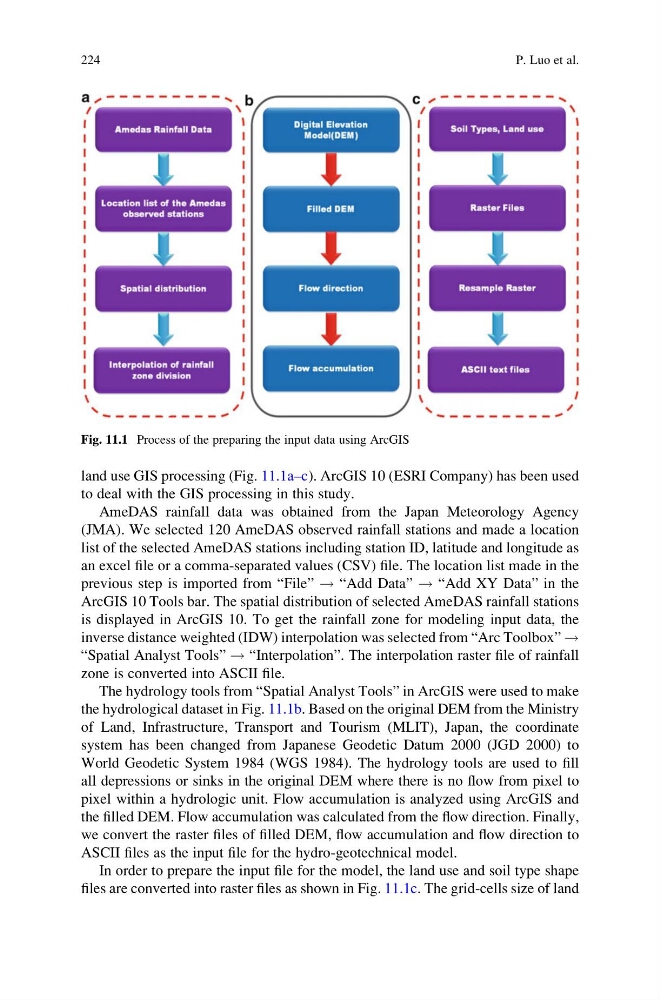
land use GIS processing (Fig. 11.1a–c). ArcGIS 10 (ESRI Company) has been used
to deal with the GIS processing in this study.
AmeDAS rainfall data was obtained from the Japan Meteorology Agency
(JMA). We selected 120 AmeDAS observed rainfall stations and made a location
list of the selected AmeDAS stations including station ID, latitude and longitude as
an excel file or a comma-separated values (CSV) file. The location list made in the
previous step is imported from “File” ! “Add Data” ! “Add XY Data” in the
ArcGIS 10 Tools bar. The spatial distribution of selected AmeDAS rainfall stations
is displayed in ArcGIS 10. To get the rainfall zone for modeling input data, the
inverse distance weighted (IDW) interpolation was selected from “Arc Toolbox” !
“Spatial Analyst Tools” ! “Interpolation”. The interpolation raster file of rainfall
zone is converted into ASCII file.
The hydrology tools from “Spatial Analyst Tools” in ArcGIS were used to make
the hydrological dataset in Fig. 11.1b. Based on the original DEM from the Ministry
of Land, Infrastructure, Transport and Tourism (MLIT), Japan, the coordinate
system has been changed from Japanese Geodetic Datum 2000 (JGD 2000) to
World Geodetic System 1984 (WGS 1984). The hydrology tools are used to fill
all depressions or sinks in the original DEM where there is no flow from pixel to
pixel within a hydrologic unit. Flow accumulation is analyzed using ArcGIS and
the filled DEM. Flow accumulation was calculated from the flow direction. Finally,
we convert the raster files of filled DEM, flow accumulation and flow direction to
ASCII files as the input file for the hydro-geotechnical model.
In order to prepare the input file for the model, the land use and soil type shape
files are converted into raster files as shown in Fig. 11.1c. The grid-cells size of land
Fig. 11.1 Process of the preparing the input data using ArcGIS
224
P. Luo et al.
to deal with the GIS processing in this study.
AmeDAS rainfall data was obtained from the Japan Meteorology Agency
(JMA). We selected 120 AmeDAS observed rainfall stations and made a location
list of the selected AmeDAS stations including station ID, latitude and longitude as
an excel file or a comma-separated values (CSV) file. The location list made in the
previous step is imported from “File” ! “Add Data” ! “Add XY Data” in the
ArcGIS 10 Tools bar. The spatial distribution of selected AmeDAS rainfall stations
is displayed in ArcGIS 10. To get the rainfall zone for modeling input data, the
inverse distance weighted (IDW) interpolation was selected from “Arc Toolbox” !
“Spatial Analyst Tools” ! “Interpolation”. The interpolation raster file of rainfall
zone is converted into ASCII file.
The hydrology tools from “Spatial Analyst Tools” in ArcGIS were used to make
the hydrological dataset in Fig. 11.1b. Based on the original DEM from the Ministry
of Land, Infrastructure, Transport and Tourism (MLIT), Japan, the coordinate
system has been changed from Japanese Geodetic Datum 2000 (JGD 2000) to
World Geodetic System 1984 (WGS 1984). The hydrology tools are used to fill
all depressions or sinks in the original DEM where there is no flow from pixel to
pixel within a hydrologic unit. Flow accumulation is analyzed using ArcGIS and
the filled DEM. Flow accumulation was calculated from the flow direction. Finally,
we convert the raster files of filled DEM, flow accumulation and flow direction to
ASCII files as the input file for the hydro-geotechnical model.
In order to prepare the input file for the model, the land use and soil type shape
files are converted into raster files as shown in Fig. 11.1c. The grid-cells size of land
Fig. 11.1 Process of the preparing the input data using ArcGIS
224
P. Luo et al.