

Y ¼ y 1 ; y 2 ; . . . ; y N
½
T
ð6:10Þ
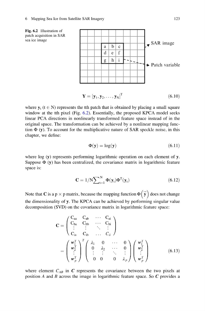
where y t (t 2 N) represents the tth patch that is obtained by placing a small square
window at the tth pixel (Fig. 6.2). Essentially, the proposed KPCA model seeks
linear PCA directions in nonlinearly transformed feature space instead of in the
original space. The transformation can be achieved by a nonlinear mapping function Φ (y). To account for the multiplicative nature of SAR speckle noise, in this
chapter, we define:
Φ y
ð Þ ¼ log y
ð Þ
ð6:11Þ
where log (y) represents performing logarithmic operation on each element of y.
Suppose Φ (y) has been centralized, the covariance matrix in logarithmic feature
space is:
C ¼ 1=N
X N
t¼1
Φ y t
ð ÞΦ
T y t
ð Þ
ð6:12Þ
Note that C is a p  p matrix, because the mapping function Φ y
!
does not change
the dimensionality of y. The KPCA can be achieved by performing singular value
decomposition (SVD) on the covariance matrix in logarithmic feature space:
C ¼
C aa C ab Á Á Á C ai
C ba C bb Á Á Á C bi
⋮
C ia
⋮
C ib
⋱ ⋮
. . . C ii
0
B
@
1
C
A
¼
w
T
1
w
T
2
⋮
w
T
p
0
B
B
@
1
C
C
A
T
λ 1
0
0
λ 2
Á Á Á
Á Á Á
0
0
⋮ ⋮
⋱ ⋮
0 0
0 λ p
0
B
B
@
1
C
C
A
w
T
1
w
T
2
⋮
w
T
p
0
B
B
@
1
C
C
A
ð6:13Þ
where element C AB in C represents the covariance between the two pixels at
position A and B across the image in logarithmic feature space. So C provides a
a b c
d e f
g
SAR image
Patch variable
h i
Fig. 6.2 Illustration of
patch acquisition in SAR
sea ice image
6 Mapping Sea Ice from Satellite SAR Imagery
123
½
T
ð6:10Þ
where y t (t 2 N) represents the tth patch that is obtained by placing a small square
window at the tth pixel (Fig. 6.2). Essentially, the proposed KPCA model seeks
linear PCA directions in nonlinearly transformed feature space instead of in the
original space. The transformation can be achieved by a nonlinear mapping function Φ (y). To account for the multiplicative nature of SAR speckle noise, in this
chapter, we define:
Φ y
ð Þ ¼ log y
ð Þ
ð6:11Þ
where log (y) represents performing logarithmic operation on each element of y.
Suppose Φ (y) has been centralized, the covariance matrix in logarithmic feature
space is:
C ¼ 1=N
X N
t¼1
Φ y t
ð ÞΦ
T y t
ð Þ
ð6:12Þ
Note that C is a p  p matrix, because the mapping function Φ y
!
does not change
the dimensionality of y. The KPCA can be achieved by performing singular value
decomposition (SVD) on the covariance matrix in logarithmic feature space:
C ¼
C aa C ab Á Á Á C ai
C ba C bb Á Á Á C bi
⋮
C ia
⋮
C ib
⋱ ⋮
. . . C ii
0
B
@
1
C
A
¼
w
T
1
w
T
2
⋮
w
T
p
0
B
B
@
1
C
C
A
T
λ 1
0
0
λ 2
Á Á Á
Á Á Á
0
0
⋮ ⋮
⋱ ⋮
0 0
0 λ p
0
B
B
@
1
C
C
A
w
T
1
w
T
2
⋮
w
T
p
0
B
B
@
1
C
C
A
ð6:13Þ
where element C AB in C represents the covariance between the two pixels at
position A and B across the image in logarithmic feature space. So C provides a
a b c
d e f
g
SAR image
Patch variable
h i
Fig. 6.2 Illustration of
patch acquisition in SAR
sea ice image
6 Mapping Sea Ice from Satellite SAR Imagery
123