

that the null hypothesis is true. It confirms whether the components of the
regression line are statistically significant. P-value < 0,01, < 0,05, or < 0,1 are
usually used as significant (Sykes 1992).
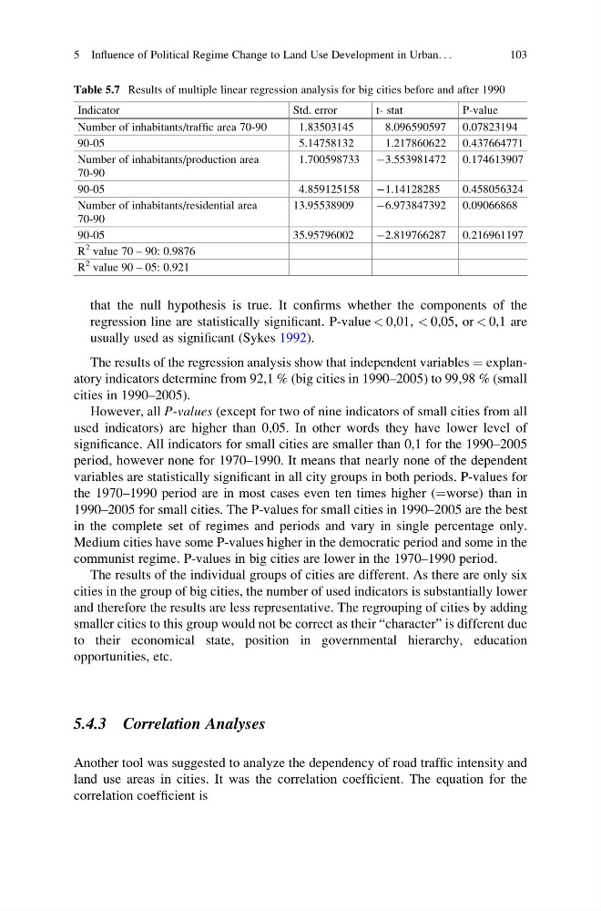
The results of the regression analysis show that independent variables ¼ explanatory indicators determine from 92,1 % (big cities in 1990–2005) to 99,98 % (small
cities in 1990–2005).
However, all P-values (except for two of nine indicators of small cities from all
used indicators) are higher than 0,05. In other words they have lower level of
significance. All indicators for small cities are smaller than 0,1 for the 1990–2005
period, however none for 1970–1990. It means that nearly none of the dependent
variables are statistically significant in all city groups in both periods. P-values for
the 1970–1990 period are in most cases even ten times higher (¼worse) than in
1990–2005 for small cities. The P-values for small cities in 1990–2005 are the best
in the complete set of regimes and periods and vary in single percentage only.
Medium cities have some P-values higher in the democratic period and some in the
communist regime. P-values in big cities are lower in the 1970–1990 period.
The results of the individual groups of cities are different. As there are only six
cities in the group of big cities, the number of used indicators is substantially lower
and therefore the results are less representative. The regrouping of cities by adding
smaller cities to this group would not be correct as their “character” is different due
to their economical state, position in governmental hierarchy, education
opportunities, etc.
5.4.3 Correlation Analyses
Another tool was suggested to analyze the dependency of road traffic intensity and
land use areas in cities. It was the correlation coefficient. The equation for the
correlation coefficient is
Table 5.7 Results of multiple linear regression analysis for big cities before and after 1990
Indicator
Std. error
t- stat
P-value
Number of inhabitants/traffic area 70-90
1.83503145
8.096590597 0.07823194
90-05
5.14758132
1.217860622 0.437664771
Number of inhabitants/production area
70-90
1.700598733 À3.553981472 0.174613907
90-05
4.859125158 À1.14128285
0.458056324
Number of inhabitants/residential area
70-90
13.95538909
À6.973847392 0.09066868
90-05
35.95796002
À2.819766287 0.216961197
R
2 value 70 – 90: 0.9876
R
2 value 90 – 05: 0.921
5 Influence of Political Regime Change to Land Use Development in Urban. . .
103
regression line are statistically significant. P-value < 0,01, < 0,05, or < 0,1 are
usually used as significant (Sykes 1992).
The results of the regression analysis show that independent variables ¼ explanatory indicators determine from 92,1 % (big cities in 1990–2005) to 99,98 % (small
cities in 1990–2005).
However, all P-values (except for two of nine indicators of small cities from all
used indicators) are higher than 0,05. In other words they have lower level of
significance. All indicators for small cities are smaller than 0,1 for the 1990–2005
period, however none for 1970–1990. It means that nearly none of the dependent
variables are statistically significant in all city groups in both periods. P-values for
the 1970–1990 period are in most cases even ten times higher (¼worse) than in
1990–2005 for small cities. The P-values for small cities in 1990–2005 are the best
in the complete set of regimes and periods and vary in single percentage only.
Medium cities have some P-values higher in the democratic period and some in the
communist regime. P-values in big cities are lower in the 1970–1990 period.
The results of the individual groups of cities are different. As there are only six
cities in the group of big cities, the number of used indicators is substantially lower
and therefore the results are less representative. The regrouping of cities by adding
smaller cities to this group would not be correct as their “character” is different due
to their economical state, position in governmental hierarchy, education
opportunities, etc.
5.4.3 Correlation Analyses
Another tool was suggested to analyze the dependency of road traffic intensity and
land use areas in cities. It was the correlation coefficient. The equation for the
correlation coefficient is
Table 5.7 Results of multiple linear regression analysis for big cities before and after 1990
Indicator
Std. error
t- stat
P-value
Number of inhabitants/traffic area 70-90
1.83503145
8.096590597 0.07823194
90-05
5.14758132
1.217860622 0.437664771
Number of inhabitants/production area
70-90
1.700598733 À3.553981472 0.174613907
90-05
4.859125158 À1.14128285
0.458056324
Number of inhabitants/residential area
70-90
13.95538909
À6.973847392 0.09066868
90-05
35.95796002
À2.819766287 0.216961197
R
2 value 70 – 90: 0.9876
R
2 value 90 – 05: 0.921
5 Influence of Political Regime Change to Land Use Development in Urban. . .
103