

126
Mapping to ‘Real World’ Objects
The process of image analysis used is known as Object Based Image Analysis
(OBIA) (Lucas et al. 2007) and eCognition image processing software (eCognition)
was used. Pixels with similar spectral characteristics were grouped into objects, with
the user defining their spectral characteristics, size and shape (Burnett and Blaschke
2003; Karl and Maurer 2010). For Norfolk, a multi-resolution -stage ‘segmentation –
classification – re-segmentation’ approach was used where large ‘woodland’ and
‘field-sized’ objects were firstly delineated and classified. Then, the image was
re-segmented within these boundaries to delineate and classify smaller, irregularlyshaped polygons which were commensurate in dimensions and geometry with the
vegetation patches within the various communities. Within this project, each object
needed to comprise at least five pixels of the remote sensing data to give sufficient
statistical validity to describe the object accurately according to Blaschke et al.
(2008). The spatial scale of the features and imagery therefore drive the image
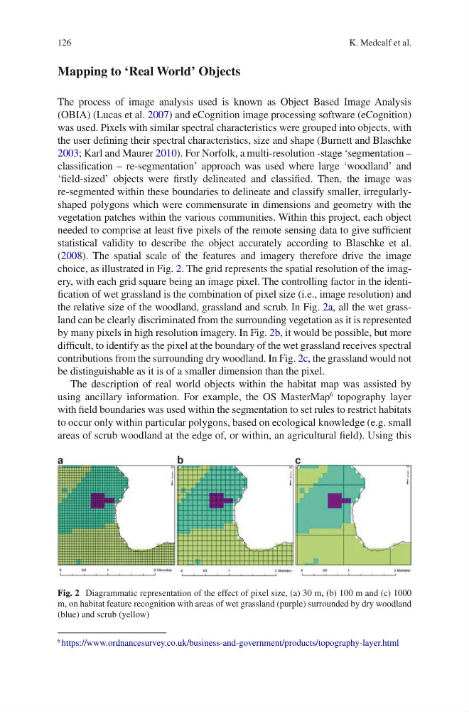
choice, as illustrated in Fig. 2. The grid represents the spatial resolution of the imagery, with each grid square being an image pixel. The controlling factor in the identification of wet grassland is the combination of pixel size (i.e., image resolution) and
the relative size of the woodland, grassland and scrub. In Fig. 2a, all the wet grassland can be clearly discriminated from the surrounding vegetation as it is represented
by many pixels in high resolution imagery. In Fig. 2b, it would be possible, but more
difficult, to identify as the pixel at the boundary of the wet grassland receives spectral
contributions from the surrounding dry woodland. In Fig. 2c, the grassland would not
be distinguishable as it is of a smaller dimension than the pixel.
The description of real world objects within the habitat map was assisted by
using ancillary information. For example, the OS MasterMap
6
topography layer
with field boundaries was used within the segmentation to set rules to restrict habitats
to occur only within particular polygons, based on ecological knowledge (e.g. small
areas of scrub woodland at the edge of, or within, an agricultural field). Using this
6 https://www.ordnancesurvey.co.uk/business-and-government/products/topography-layer.html
Fig. 2 Diagrammatic representation of the effect of pixel size, (a) 30 m, (b) 100 m and (c) 1000
m, on habitat feature recognition with areas of wet grassland (purple) surrounded by dry woodland
(blue) and scrub (yellow)
K. Medcalf et al.
Mapping to ‘Real World’ Objects
The process of image analysis used is known as Object Based Image Analysis
(OBIA) (Lucas et al. 2007) and eCognition image processing software (eCognition)
was used. Pixels with similar spectral characteristics were grouped into objects, with
the user defining their spectral characteristics, size and shape (Burnett and Blaschke
2003; Karl and Maurer 2010). For Norfolk, a multi-resolution -stage ‘segmentation –
classification – re-segmentation’ approach was used where large ‘woodland’ and
‘field-sized’ objects were firstly delineated and classified. Then, the image was
re-segmented within these boundaries to delineate and classify smaller, irregularlyshaped polygons which were commensurate in dimensions and geometry with the
vegetation patches within the various communities. Within this project, each object
needed to comprise at least five pixels of the remote sensing data to give sufficient
statistical validity to describe the object accurately according to Blaschke et al.
(2008). The spatial scale of the features and imagery therefore drive the image
choice, as illustrated in Fig. 2. The grid represents the spatial resolution of the imagery, with each grid square being an image pixel. The controlling factor in the identification of wet grassland is the combination of pixel size (i.e., image resolution) and
the relative size of the woodland, grassland and scrub. In Fig. 2a, all the wet grassland can be clearly discriminated from the surrounding vegetation as it is represented
by many pixels in high resolution imagery. In Fig. 2b, it would be possible, but more
difficult, to identify as the pixel at the boundary of the wet grassland receives spectral
contributions from the surrounding dry woodland. In Fig. 2c, the grassland would not
be distinguishable as it is of a smaller dimension than the pixel.
The description of real world objects within the habitat map was assisted by
using ancillary information. For example, the OS MasterMap
6
topography layer
with field boundaries was used within the segmentation to set rules to restrict habitats
to occur only within particular polygons, based on ecological knowledge (e.g. small
areas of scrub woodland at the edge of, or within, an agricultural field). Using this
6 https://www.ordnancesurvey.co.uk/business-and-government/products/topography-layer.html
Fig. 2 Diagrammatic representation of the effect of pixel size, (a) 30 m, (b) 100 m and (c) 1000
m, on habitat feature recognition with areas of wet grassland (purple) surrounded by dry woodland
(blue) and scrub (yellow)
K. Medcalf et al.