

5 Model Generalization
89
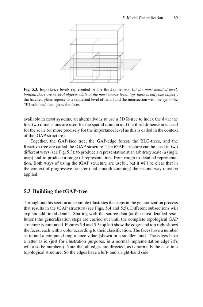
Fig. 5.3. Importance levels represented by the third dimension (at the most detailed level,
bottom, there are several objects while at the most coarse level, top, there is only one object);
the hatched plane represents a requested level of detail and the intersection with the symbolic
‘3D volumes’ then gives the faces
available in most systems, an alternative is to use a 3D R-tree to index the data: the
first two dimensions are used for the spatial domain and the third dimension is used
for the scale (or more precisely for the importance level as this is called in the context
of the tGAP structure).
Together, the GAP-face tree, the GAP-edge forest, the BLG-trees, and the
Reactive-tree are called the tGAP structure. The tGAP structure can be used in two
different ways (see Fig. 5.3): to produce a representation at an arbitrary scale (a single
map) and to produce a range of representations from rough to detailed representation. Both ways of using the tGAP structure are useful, but it will be clear that in
the context of progressive transfer (and smooth zooming) the second way must be
applied.
5.3 Building the tGAP-tree
Throughout this section an example illustrates the steps in the generalization process
that results in the tGAP structure (see Figs. 5.4 and 5.5). Different subsections will
explain additional details. Starting with the source data (at the most detailed resolution) the generalization steps are carried out until the complete topological GAP
structure is computed. Figures 5.4 and 5.5 top left show the edges and top right shows
the faces, each with a color according to their classification. The faces have a number
as id and a computed importance value (shown in a smaller font). The edges have
a letter as id (just for illustration purposes, in a normal implementation edge id’s
will also be numbers). Note that all edges are directed, as is normally the case in a
topological structure. So the edges have a left- and a right-hand side.
89
Fig. 5.3. Importance levels represented by the third dimension (at the most detailed level,
bottom, there are several objects while at the most coarse level, top, there is only one object);
the hatched plane represents a requested level of detail and the intersection with the symbolic
‘3D volumes’ then gives the faces
available in most systems, an alternative is to use a 3D R-tree to index the data: the
first two dimensions are used for the spatial domain and the third dimension is used
for the scale (or more precisely for the importance level as this is called in the context
of the tGAP structure).
Together, the GAP-face tree, the GAP-edge forest, the BLG-trees, and the
Reactive-tree are called the tGAP structure. The tGAP structure can be used in two
different ways (see Fig. 5.3): to produce a representation at an arbitrary scale (a single
map) and to produce a range of representations from rough to detailed representation. Both ways of using the tGAP structure are useful, but it will be clear that in
the context of progressive transfer (and smooth zooming) the second way must be
applied.
5.3 Building the tGAP-tree
Throughout this section an example illustrates the steps in the generalization process
that results in the tGAP structure (see Figs. 5.4 and 5.5). Different subsections will
explain additional details. Starting with the source data (at the most detailed resolution) the generalization steps are carried out until the complete topological GAP
structure is computed. Figures 5.4 and 5.5 top left show the edges and top right shows
the faces, each with a color according to their classification. The faces have a number
as id and a computed importance value (shown in a smaller font). The edges have
a letter as id (just for illustration purposes, in a normal implementation edge id’s
will also be numbers). Note that all edges are directed, as is normally the case in a
topological structure. So the edges have a left- and a right-hand side.