

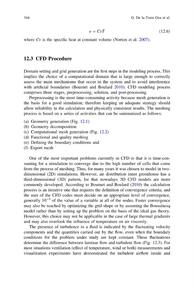
e ¼ CvT
ð12:6Þ
where Cv is the specific heat at constant volume (Norton et al. 2007).
12.3 CFD Procedure
Domain setting and grid generation are the first steps in the modeling process. This
implies the choice of a computational domain that is large enough to correctly
assess the main mechanisms that occur in the system and to avoid interference
with artificial boundaries (Bournet and Boulard 2010). CFD modeling process
comprises three stages, preprocessing, solution, and post-processing.
Preprocessing is the most time-consuming activity because mesh generation is
the basis for a good simulation; therefore keeping an adequate strategy should
allow reliability in the calculation and physically consistent results. The meshing
process is based on a series of activities that can be summarized as follows:
(a) Geometry generation (Fig. 12.1)
(b) Geometry decomposition
(c) Computational mesh generation (Fig. 12.2)
(d) Functional and quality meshing
(e) Defining the boundary conditions and
(f) Export mesh
One of the most important problems currently in CFD is that it is time-consuming for a simulation to converge due to the high number of cells that come
from the process of meshing. Thus, for many years it was chosen to model in twodimensional (2D) simulations. However, air distribution inner greenhouse has a
third-dimensional (3D) pattern, for that nowadays 3D CFD models are more
commonly developed. According to Bournet and Boulard (2010) the calculation
process is an iterative one that requires the definition of convergence criteria, and
the user of the CFD codes must decide on an appropriate level of convergence,
generally 10
-4 of the value of a variable at all of the nodes. Faster convergence
may also be reached by optimizing the grid shape or by assuming the Boussinesq
model rather than by setting up the problem on the basis of the ideal gas theory.
However, this choice may not be applicable in the case of large thermal gradients
and may also overlook the influence of temperature on air viscosity.
The presence of turbulence in a fluid is indicated by the fluctuating velocity
components and the quantities carried out by the flow, even when the boundary
conditions for the problem under study are kept constant. These fluctuations
determine the difference between laminar flow and turbulent flow (Fig. 12.3). For
most situations ventilation (effect of temperature, wind or both) measurements and
visualization experiments have demonstrated the turbulent airflow inside and
344
G. De la Torre-Gea et al.
ð12:6Þ
where Cv is the specific heat at constant volume (Norton et al. 2007).
12.3 CFD Procedure
Domain setting and grid generation are the first steps in the modeling process. This
implies the choice of a computational domain that is large enough to correctly
assess the main mechanisms that occur in the system and to avoid interference
with artificial boundaries (Bournet and Boulard 2010). CFD modeling process
comprises three stages, preprocessing, solution, and post-processing.
Preprocessing is the most time-consuming activity because mesh generation is
the basis for a good simulation; therefore keeping an adequate strategy should
allow reliability in the calculation and physically consistent results. The meshing
process is based on a series of activities that can be summarized as follows:
(a) Geometry generation (Fig. 12.1)
(b) Geometry decomposition
(c) Computational mesh generation (Fig. 12.2)
(d) Functional and quality meshing
(e) Defining the boundary conditions and
(f) Export mesh
One of the most important problems currently in CFD is that it is time-consuming for a simulation to converge due to the high number of cells that come
from the process of meshing. Thus, for many years it was chosen to model in twodimensional (2D) simulations. However, air distribution inner greenhouse has a
third-dimensional (3D) pattern, for that nowadays 3D CFD models are more
commonly developed. According to Bournet and Boulard (2010) the calculation
process is an iterative one that requires the definition of convergence criteria, and
the user of the CFD codes must decide on an appropriate level of convergence,
generally 10
-4 of the value of a variable at all of the nodes. Faster convergence
may also be reached by optimizing the grid shape or by assuming the Boussinesq
model rather than by setting up the problem on the basis of the ideal gas theory.
However, this choice may not be applicable in the case of large thermal gradients
and may also overlook the influence of temperature on air viscosity.
The presence of turbulence in a fluid is indicated by the fluctuating velocity
components and the quantities carried out by the flow, even when the boundary
conditions for the problem under study are kept constant. These fluctuations
determine the difference between laminar flow and turbulent flow (Fig. 12.3). For
most situations ventilation (effect of temperature, wind or both) measurements and
visualization experiments have demonstrated the turbulent airflow inside and
344
G. De la Torre-Gea et al.