

102
L. G.-Weil et al.
But this is not the only way that eddies are detected in SST and Chl-a scenes.
Another possibility is that water with different surface SST and/or Chl-a properties
can be wrapped around the eddies’ core. Then, SST and Chl-a can be considered
as tracers of the water flow. This mechanism of eddy observation is useful when
large scale gradients of SST an Chl-a, like those observed frequently in the coastal
transition zone, are present. As it will be shown in next section, the signal of ocean
eddies in the SST and Chl-a fields disappears, albeit not at the same time, when
they move away from the coastal transition zone and into offshore areas. This is
produced because of the intensity decay of eddies and the simultaneous weakening
of the surface gradients of SST and Chl-a fields. The signal of the eddies usually lasts
for a longer time in SLA maps, as in Fig. 5.1d, again this being a property directly
related to ocean dynamics.
5.3 Mesoscale Variability in the Canary Islands Area
5.3.1 Annual and Seasonal Characteristics of Mesoscale Activity
The eddy kinetic energy, drawn from the SLA-derived geostrophic velocity
anomalies, i.e.
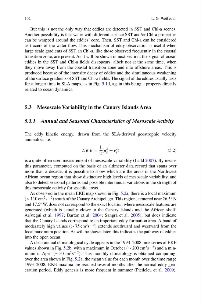
EKE =
1
2
(u
2
g + v
2
g )
(5.2)
is a quite often used measurement of mesoscale variability (Ladd 2007). By means
this parameter, computed on the basis of an altimeter data record that spans over
more than a decade, it is possible to show which are the areas in the Northwest
African ocean region that show distinctive high levels of mesoscale variability, and
also to detect seasonal patterns and possible interannual variations in the strength of
this mesoscale activity for specific areas.
As observed in the mean EKE map shown in Fig. 5.2a, there is a local maximum
(> 110 cm
2 s
− 2 ) south of the Canary Archipelago. This region, centered near 26.5
◦ N
and 17.5
◦ W, does not correspond to the exact location where mesoscale features are
generated (which is actually closer to the Canary Islands and the African shelf;
Arístegui et al. 1997; Barton et al. 2004; Sangrà et al. 2005), but does indicate
that the Canary Islands correspond to an important eddy formation area. A band of
moderately high values (> 75 cm
2 s
− 2 ) extends southward and westward from the
local maximum position. As will be shown later, this indicates the pathway of eddies
into the open ocean.
A clear annual climatological cycle appears in the 1993–2008 time series of EKE
values shown in Fig. 5.2b, with a maximum in October (∼ 200 cm
2 s
− 2 ) and a minimum in April (∼ 50 cm
2 s
− 2 ). This monthly climatology is obtained computing,
over the area shown in Fig. 5.2a, the mean value for each month over the time range
1993–2008. EKE maxima are reached several months after the normal eddy generation period. Eddy genesis is more frequent in summer (Piedeleu et al. 2009),
L. G.-Weil et al.
But this is not the only way that eddies are detected in SST and Chl-a scenes.
Another possibility is that water with different surface SST and/or Chl-a properties
can be wrapped around the eddies’ core. Then, SST and Chl-a can be considered
as tracers of the water flow. This mechanism of eddy observation is useful when
large scale gradients of SST an Chl-a, like those observed frequently in the coastal
transition zone, are present. As it will be shown in next section, the signal of ocean
eddies in the SST and Chl-a fields disappears, albeit not at the same time, when
they move away from the coastal transition zone and into offshore areas. This is
produced because of the intensity decay of eddies and the simultaneous weakening
of the surface gradients of SST and Chl-a fields. The signal of the eddies usually lasts
for a longer time in SLA maps, as in Fig. 5.1d, again this being a property directly
related to ocean dynamics.
5.3 Mesoscale Variability in the Canary Islands Area
5.3.1 Annual and Seasonal Characteristics of Mesoscale Activity
The eddy kinetic energy, drawn from the SLA-derived geostrophic velocity
anomalies, i.e.
EKE =
1
2
(u
2
g + v
2
g )
(5.2)
is a quite often used measurement of mesoscale variability (Ladd 2007). By means
this parameter, computed on the basis of an altimeter data record that spans over
more than a decade, it is possible to show which are the areas in the Northwest
African ocean region that show distinctive high levels of mesoscale variability, and
also to detect seasonal patterns and possible interannual variations in the strength of
this mesoscale activity for specific areas.
As observed in the mean EKE map shown in Fig. 5.2a, there is a local maximum
(> 110 cm
2 s
− 2 ) south of the Canary Archipelago. This region, centered near 26.5
◦ N
and 17.5
◦ W, does not correspond to the exact location where mesoscale features are
generated (which is actually closer to the Canary Islands and the African shelf;
Arístegui et al. 1997; Barton et al. 2004; Sangrà et al. 2005), but does indicate
that the Canary Islands correspond to an important eddy formation area. A band of
moderately high values (> 75 cm
2 s
− 2 ) extends southward and westward from the
local maximum position. As will be shown later, this indicates the pathway of eddies
into the open ocean.
A clear annual climatological cycle appears in the 1993–2008 time series of EKE
values shown in Fig. 5.2b, with a maximum in October (∼ 200 cm
2 s
− 2 ) and a minimum in April (∼ 50 cm
2 s
− 2 ). This monthly climatology is obtained computing,
over the area shown in Fig. 5.2a, the mean value for each month over the time range
1993–2008. EKE maxima are reached several months after the normal eddy generation period. Eddy genesis is more frequent in summer (Piedeleu et al. 2009),