

34
2. Modeling in STELLA
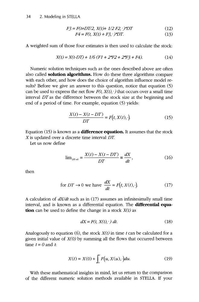
Fj =F(t+DTI2, xo» 112F2, YDT
F4
(12)
(13)
A weighted sum of those four estimates is then used to calculate the stock:
X(t) =X(t-DT) + 116(Fl + 2*F2 + 2*Fj +F4).
(14)
Numeric solution techniques such as the ones described above are often
also called solution algorithms. How do these three algorithms compare
with each other, and how does the choice of algorithm influence model results? Before we give an answer to this question, notice that equation (5)
can be used to express the net flow FO, Xtt), -) that occurs over a small time
interval DT as the difference between the stock size at the beginning and
end of a period of time. For example, equation (5) yields:
XU) - X(t - DT) = F(t, X(t) ,-).
DT
(15)
Equation (15) is known as a difference equation. It assumes that the stock
X is updated over a discrete time interval DT.
Let us now define
lim
DT-->O
= X(t) - X(t - DT) == dX
DT
dt '
(16)
then
dX
for DT -) 0 we have - = F(t, XU), .).
(17)
dt
A calculation of dXldt such as in (17) assumes an infinitesimally small time
interval, and is known as a differential equation. The differential equation can be used to define the change in a stock X(t) as
dX =F(t, X(t), -) dt.
(18)
Analogously to equ ation (6) , the stock X(t) in time t can be calculated for a
given initial value of X(O) by summing all the flows that occurred between
time t =0 and t:
X ( t) = X(O) + s:F(u, X(u), -)du.
(19)
With these mathemat ical insights in mind, let us return to the comp arison
of the different numeric solution methods available in STELLA. If your
2. Modeling in STELLA
Fj =F(t+DTI2, xo» 112F2, YDT
F4
(12)
(13)
A weighted sum of those four estimates is then used to calculate the stock:
X(t) =X(t-DT) + 116(Fl + 2*F2 + 2*Fj +F4).
(14)
Numeric solution techniques such as the ones described above are often
also called solution algorithms. How do these three algorithms compare
with each other, and how does the choice of algorithm influence model results? Before we give an answer to this question, notice that equation (5)
can be used to express the net flow FO, Xtt), -) that occurs over a small time
interval DT as the difference between the stock size at the beginning and
end of a period of time. For example, equation (5) yields:
XU) - X(t - DT) = F(t, X(t) ,-).
DT
(15)
Equation (15) is known as a difference equation. It assumes that the stock
X is updated over a discrete time interval DT.
Let us now define
lim
DT-->O
= X(t) - X(t - DT) == dX
DT
dt '
(16)
then
dX
for DT -) 0 we have - = F(t, XU), .).
(17)
dt
A calculation of dXldt such as in (17) assumes an infinitesimally small time
interval, and is known as a differential equation. The differential equation can be used to define the change in a stock X(t) as
dX =F(t, X(t), -) dt.
(18)
Analogously to equ ation (6) , the stock X(t) in time t can be calculated for a
given initial value of X(O) by summing all the flows that occurred between
time t =0 and t:
X ( t) = X(O) + s:F(u, X(u), -)du.
(19)
With these mathemat ical insights in mind, let us return to the comp arison
of the different numeric solution methods available in STELLA. If your