

2.3. STELLA's Numeric Solution Techniques
33
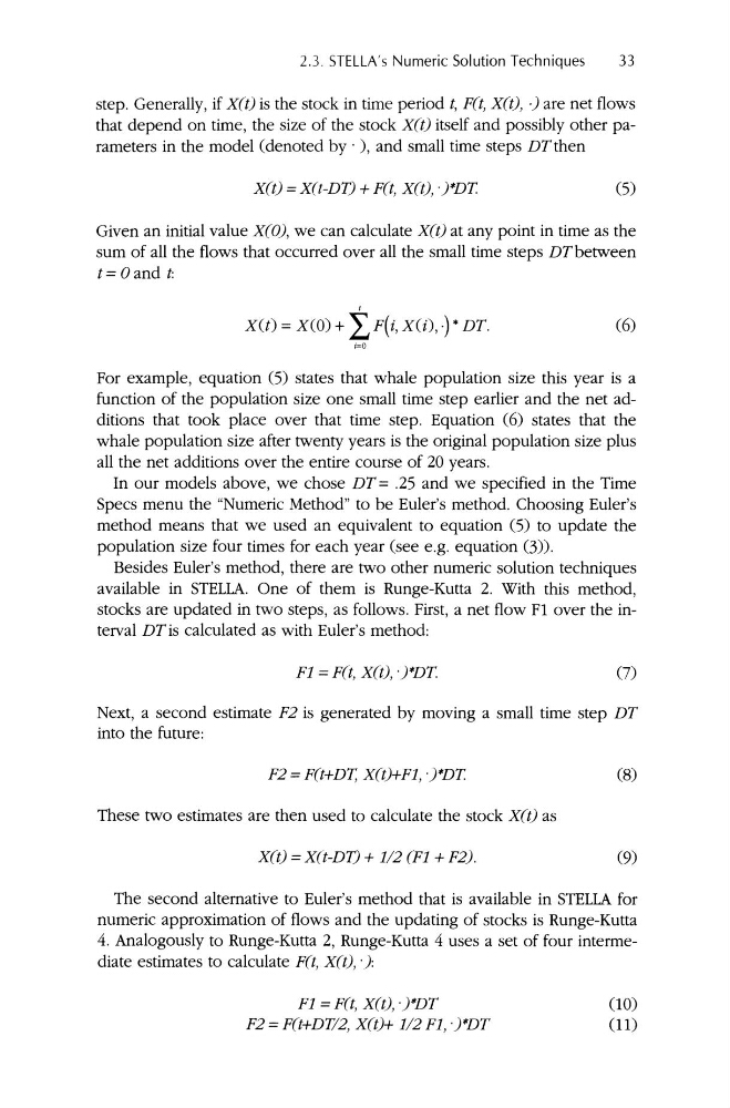
step . Generally , if X(t) is the stock in time period t, F(t, Xtt), -) are net flows
that depend on time, the size of the stock X(t) itself and possibly other parameters in the model (denoted by . ), and small time steps DTthen
X(t) = X(t-DTJ + F(t, X(t), )*DT
(5)
Given an initial value X(OJ, we can calculate X(t) at any point in time as the
sum of all the flows that occurred over all the small time steps DTbetween
t= oand t:
XU) = X(O) + ItF(i,
I
X(i), .) • DT.
j= O
(6)
For example, equation (5) states that whale population size this year is a
function of the population size one small time step earlier and the net additions that took place over that time step . Equation (6) states that the
whale population size after twenty years is the original population size plus
all the net additions over the entire course of 20 years.
In our models above , we chose DT= .25 and we specified in the Time
Specs menu the "Numeric Method" to be Euler's method. Choosing Euler's
method mean s that we used an equivalent to equation (5) to update the
population size four times for each year (see e.g. equation (3)).
Besides Euler's method, there are two other numeric solution techniques
available in STELLA. One of them is Runge-Kutta 2. With this method,
stocks are updated in two steps, as follows. First, a net flow Fl over the interval DTis calculated as with Euler's method:
F1 =F(t, X(t), )*DT.
(7)
Next, a second estimate F2 is generated by moving a small time step DT
into the future :
F2 =F(t+DT, X(t)+F1, )*DT
These two estimates are then used to calculate the stock X (t) as
X(t) =X(t-DTJ+ 1/2 (F1 + F2).
(8)
(9)
The second alternative to Euler's method that is available in STELLA for
numeric approximation of flows and the updating of stocks is Runge-Kutta
4. Analogously to Runge-Kutta 2, Runge-Kutta 4 uses a set of four intermediate estimates to calculate F(t, Xtt) , .J:
F1 =FCt, X(t), )*DT
F2 =FCt+DT/2, X(t)+ 1/2 F1, )*DT
(0)
(1)
33
step . Generally , if X(t) is the stock in time period t, F(t, Xtt), -) are net flows
that depend on time, the size of the stock X(t) itself and possibly other parameters in the model (denoted by . ), and small time steps DTthen
X(t) = X(t-DTJ + F(t, X(t), )*DT
(5)
Given an initial value X(OJ, we can calculate X(t) at any point in time as the
sum of all the flows that occurred over all the small time steps DTbetween
t= oand t:
XU) = X(O) + ItF(i,
I
X(i), .) • DT.
j= O
(6)
For example, equation (5) states that whale population size this year is a
function of the population size one small time step earlier and the net additions that took place over that time step . Equation (6) states that the
whale population size after twenty years is the original population size plus
all the net additions over the entire course of 20 years.
In our models above , we chose DT= .25 and we specified in the Time
Specs menu the "Numeric Method" to be Euler's method. Choosing Euler's
method mean s that we used an equivalent to equation (5) to update the
population size four times for each year (see e.g. equation (3)).
Besides Euler's method, there are two other numeric solution techniques
available in STELLA. One of them is Runge-Kutta 2. With this method,
stocks are updated in two steps, as follows. First, a net flow Fl over the interval DTis calculated as with Euler's method:
F1 =F(t, X(t), )*DT.
(7)
Next, a second estimate F2 is generated by moving a small time step DT
into the future :
F2 =F(t+DT, X(t)+F1, )*DT
These two estimates are then used to calculate the stock X (t) as
X(t) =X(t-DTJ+ 1/2 (F1 + F2).
(8)
(9)
The second alternative to Euler's method that is available in STELLA for
numeric approximation of flows and the updating of stocks is Runge-Kutta
4. Analogously to Runge-Kutta 2, Runge-Kutta 4 uses a set of four intermediate estimates to calculate F(t, Xtt) , .J:
F1 =FCt, X(t), )*DT
F2 =FCt+DT/2, X(t)+ 1/2 F1, )*DT
(0)
(1)