1. -1. Royer and A. Shtuka : Stochastic Imaging of Environmental Data
107
"
'"
,. . . ..
,.
,.
,.
. . . .
.. +-----L-----'---::--''-w..---/:r--+ ..
50 +---'-----'-....,....--'------;"+ ..
..
. .
. .
"
JO
,.
..
..
. .
10
,.
,.
"
,. "
,.
.. ..
, . J. ,. .. ..
,. It
I . ..
, . .. It
50
.. -I-----L-----'----'lr.'"'n:::JI'Ifo--+ It
.. +-_---L-_---'-_--'_-;;-'";-_-j- ,.
..
It
,.
. .
It
"
,. It
.. 50
"
,.
"
,.
J.
"
II
, -
It
It
,.
,. It It .. 50
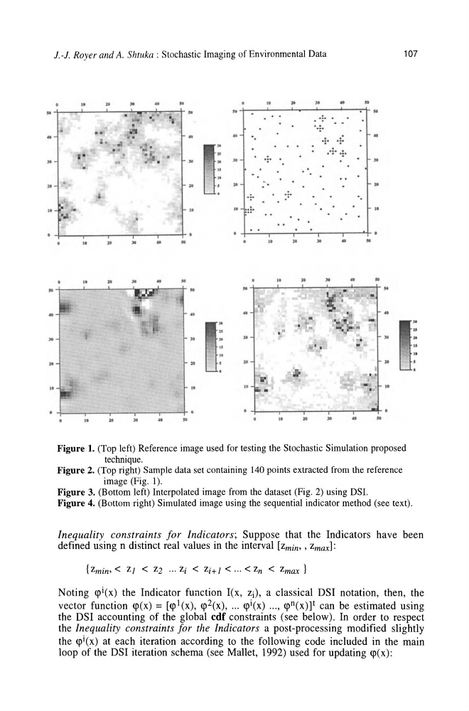
Figure 1. (Top left) Reference image used for testing the Stochastic Simulation proposed
technique.
Figure 2. (Top right) Sample data set containing 140 points extracted from the reference
image (Fig. I).
Figure 3. (Bottom left) Interpolated image from the dataset (Fig. 2) using DS!.
Figure 4. (Bottom right) Simulated image using the sequential indicator method (see text).
"
It
" II
Inequality constraints for Indicators; Suppose that the Indicators have been
defined using n distinct real values in the interval [Zmin, , zmax]:
{Zmin' < Z 1 < z2 ... zi < zi+ 1 < ... < zn < zmax }
Noting vector function the DSI accounting of the global cdC constraints (see below). In order to respect
the Inequality constraints for the Indicators a post-processing modified slightly
the loop of the DSI iteration schema (see Mallet, 1992) used for updating