

10. Acoustic Models of Sound Production
463
(A)
Z
y
1
0.8
0.6
0.4
0.2
o
(B)
=-.;-+--+---i:,.-+--Hi!llll Behind
Below
Above
(C)
0.1 ------0.2 _---0-_0.3 .---0.4 -0----0.5 ------0.6 --------0.7 --------0.8 ------0- ,
0_9 - - ;\:)
!¥:,
Behind ~'t--t--lR--f-----H;
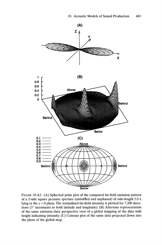
FIGURE 10.A2. (A) Spherical polar plot of the computed far-field emission pattern
of a 2-side square pressure sperture (unbaffled and unphased) of side-length 2.0 "lying in the x = 0 plane. The normalized far-field intensity is plotted for 7,200 directions (3° increments in both latitude and longitude). (B) Alternate-representation
of the same emission data: perspective view of a global mapping of the data with
height indicating intensity. (C) Contour plot of the same data projected down into
the plane of the global map.
463
(A)
Z
y
1
0.8
0.6
0.4
0.2
o
(B)
=-.;-+--+---i:,.-+--Hi!llll Behind
Below
Above
(C)
0.1 ------0.2 _---0-_0.3 .---0.4 -0----0.5 ------0.6 --------0.7 --------0.8 ------0- ,
0_9 - - ;\:)
!¥:,
Behind ~'t--t--lR--f-----H;
FIGURE 10.A2. (A) Spherical polar plot of the computed far-field emission pattern
of a 2-side square pressure sperture (unbaffled and unphased) of side-length 2.0 "lying in the x = 0 plane. The normalized far-field intensity is plotted for 7,200 directions (3° increments in both latitude and longitude). (B) Alternate-representation
of the same emission data: perspective view of a global mapping of the data with
height indicating intensity. (C) Contour plot of the same data projected down into
the plane of the global map.