

462
lL. Aroyan et al.
Appendix A
This Appendix gives the far-field form of the Helmholtz integral equation
used in the modeling of Aroyan (1996) and notes aspects of its numerical
implementation. We also illustrate a simple example of a computed far-field
pattern and introduce an efficient representation of this data over all emission directions.
It can be shown that the following expression is proportional to the farfield pressure [Eq. (3)] when R » (J [Aroyan (1996)]:
ptt(R) =f{ikR.np(eJ) + d~~eJ) }e-ikROOdSCeJ)
(AI)
where R= R/R defines the unit vector in the direction of the far-field point
(geometry diagrammed in Figure 10.2). The values of the pressure P and
the normal derivative of the pressure dp/dn over the extrapolation surfaces
were obtained from finite difference (FD) simulations. Since both the pressure and the normal derivative fields were obtained by simulation, the difficulties normally associated with nonunique solutions at eigenfrequencies
of the interior problem were not encountered. These simulated p and dp/dn
fields were then interpolated with continuous (complex bicubic) polynomials, allowing a high-order approximation to the integral (Eq. AI) to be
(A)
y
(B)
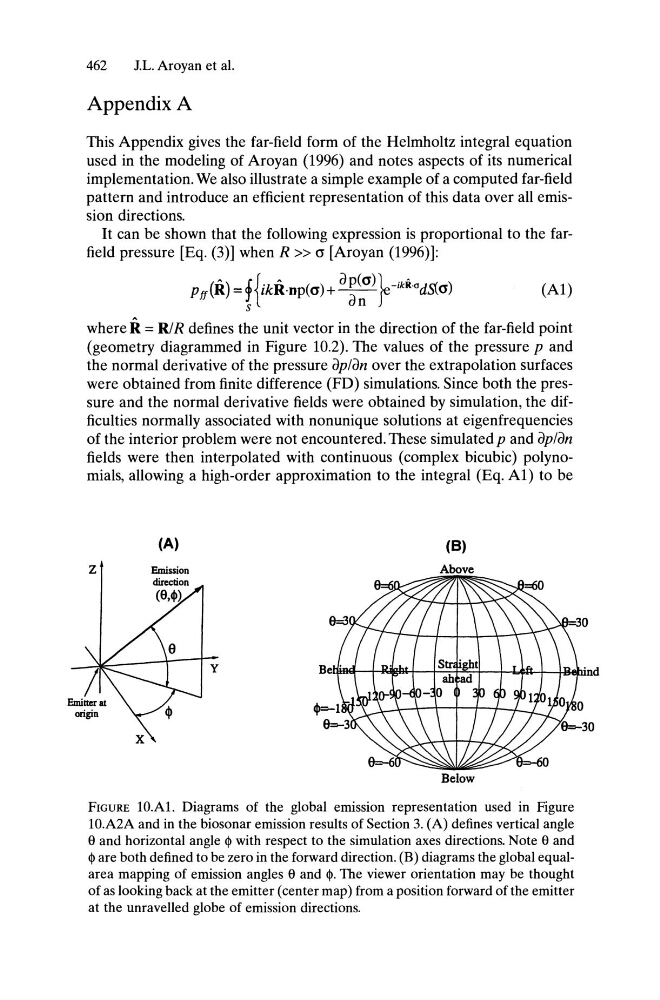
FiGURE 1O.Al. Diagrams of the global emission representation used in Figure
1O.A2A and in the biosonar emission results of Section 3. (A) defines vertical angle
8 and horizontal angle $ with respect to the simulation axes directions. Note 8 and
$ are both defined to be zero in the forward direction. (B) diagrams the global equalarea mapping of emission angles 8 and $. The viewer orientation may be thought
of as looking back at the emitter (center map) from a position forward of the emitter
at the unravelled globe of emission directions.
lL. Aroyan et al.
Appendix A
This Appendix gives the far-field form of the Helmholtz integral equation
used in the modeling of Aroyan (1996) and notes aspects of its numerical
implementation. We also illustrate a simple example of a computed far-field
pattern and introduce an efficient representation of this data over all emission directions.
It can be shown that the following expression is proportional to the farfield pressure [Eq. (3)] when R » (J [Aroyan (1996)]:
ptt(R) =f{ikR.np(eJ) + d~~eJ) }e-ikROOdSCeJ)
(AI)
where R= R/R defines the unit vector in the direction of the far-field point
(geometry diagrammed in Figure 10.2). The values of the pressure P and
the normal derivative of the pressure dp/dn over the extrapolation surfaces
were obtained from finite difference (FD) simulations. Since both the pressure and the normal derivative fields were obtained by simulation, the difficulties normally associated with nonunique solutions at eigenfrequencies
of the interior problem were not encountered. These simulated p and dp/dn
fields were then interpolated with continuous (complex bicubic) polynomials, allowing a high-order approximation to the integral (Eq. AI) to be
(A)
y
(B)
FiGURE 1O.Al. Diagrams of the global emission representation used in Figure
1O.A2A and in the biosonar emission results of Section 3. (A) defines vertical angle
8 and horizontal angle $ with respect to the simulation axes directions. Note 8 and
$ are both defined to be zero in the forward direction. (B) diagrams the global equalarea mapping of emission angles 8 and $. The viewer orientation may be thought
of as looking back at the emitter (center map) from a position forward of the emitter
at the unravelled globe of emission directions.