

(3)
414
IL. Aroyan et al.
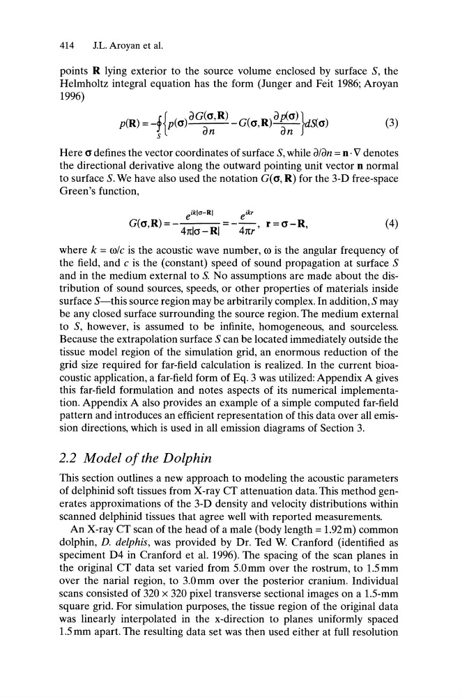
points R lying exterior to the source volume enclosed by surface S, the
Helmholtz integral equation has the form (Junger and Feit 1986; Aroyan
1996)
p(R) = -f{p(<1) aG(<1,R) -G(<1,R) a [1..(1) LS(<1)
s
an
an J
Here <1 defines the vector coordinates of surface S, while alan = n· V' denotes
the directional derivative along the outward pointing unit vector n normal
to surface S. We have also used the notation G(<1, R) for the 3-D free-space
Green's function,
(4)
where k = wle is the acoustic wave number, w is the angular frequency of
the field, and e is the (constant) speed of sound propagation at surface S
and in the medium external to S. No assumptions are made about the distribution of sound sources, speeds, or other properties of materials inside
surface S-this source region may be arbitrarily complex. In addition, S may
be any closed surface surrounding the source region. The medium external
to S, however, is assumed to be infinite, homogeneous, and sourceless.
Because the extrapolation surface S can be located immediately outside the
tissue model region of the simulation grid, an enormous reduction of the
grid size required for far-field calculation is realized. In the current bioacoustic application, a far-field form of Eq. 3 was utilized: Appendix A gives
this far-field formulation and notes aspects of its numerical implementation. Appendix A also provides an example of a simple computed far-field
pattern and introduces an efficient representation of this data over all emission directions, which is used in all emission diagrams of Section 3.
2.2 Model of the Dolphin
This section outlines a new approach to modeling the acoustic parameters
of delphinid soft tissues from X-ray CT attenuation data. This method generates approximations of the 3-D density and velocity distributions within
scanned delphinid tissues that agree well with reported measurements.
An X-ray CT scan of the head of a male (body length = 1.92m) common
dolphin, D. de/phis, was provided by Dr. Ted W. Cranford (identified as
speciment D4 in Cranford et al. 1996). The spacing of the scan planes in
the original CT data set varied from 5.0mm over the rostrum, to 1.5mm
over the narial region, to 3.0mm over the posterior cranium. Individual
scans consisted of 320 x 320 pixel transverse sectional images on a 1.5-mm
square grid. For simulation purposes, the tissue region of the original data
was linearly interpolated in the x-direction to planes uniformly spaced
1.5 mm apart. The resulting data set was then used either at full resolution
414
IL. Aroyan et al.
points R lying exterior to the source volume enclosed by surface S, the
Helmholtz integral equation has the form (Junger and Feit 1986; Aroyan
1996)
p(R) = -f{p(<1) aG(<1,R) -G(<1,R) a [1..(1) LS(<1)
s
an
an J
Here <1 defines the vector coordinates of surface S, while alan = n· V' denotes
the directional derivative along the outward pointing unit vector n normal
to surface S. We have also used the notation G(<1, R) for the 3-D free-space
Green's function,
(4)
where k = wle is the acoustic wave number, w is the angular frequency of
the field, and e is the (constant) speed of sound propagation at surface S
and in the medium external to S. No assumptions are made about the distribution of sound sources, speeds, or other properties of materials inside
surface S-this source region may be arbitrarily complex. In addition, S may
be any closed surface surrounding the source region. The medium external
to S, however, is assumed to be infinite, homogeneous, and sourceless.
Because the extrapolation surface S can be located immediately outside the
tissue model region of the simulation grid, an enormous reduction of the
grid size required for far-field calculation is realized. In the current bioacoustic application, a far-field form of Eq. 3 was utilized: Appendix A gives
this far-field formulation and notes aspects of its numerical implementation. Appendix A also provides an example of a simple computed far-field
pattern and introduces an efficient representation of this data over all emission directions, which is used in all emission diagrams of Section 3.
2.2 Model of the Dolphin
This section outlines a new approach to modeling the acoustic parameters
of delphinid soft tissues from X-ray CT attenuation data. This method generates approximations of the 3-D density and velocity distributions within
scanned delphinid tissues that agree well with reported measurements.
An X-ray CT scan of the head of a male (body length = 1.92m) common
dolphin, D. de/phis, was provided by Dr. Ted W. Cranford (identified as
speciment D4 in Cranford et al. 1996). The spacing of the scan planes in
the original CT data set varied from 5.0mm over the rostrum, to 1.5mm
over the narial region, to 3.0mm over the posterior cranium. Individual
scans consisted of 320 x 320 pixel transverse sectional images on a 1.5-mm
square grid. For simulation purposes, the tissue region of the original data
was linearly interpolated in the x-direction to planes uniformly spaced
1.5 mm apart. The resulting data set was then used either at full resolution