

244
Appendices
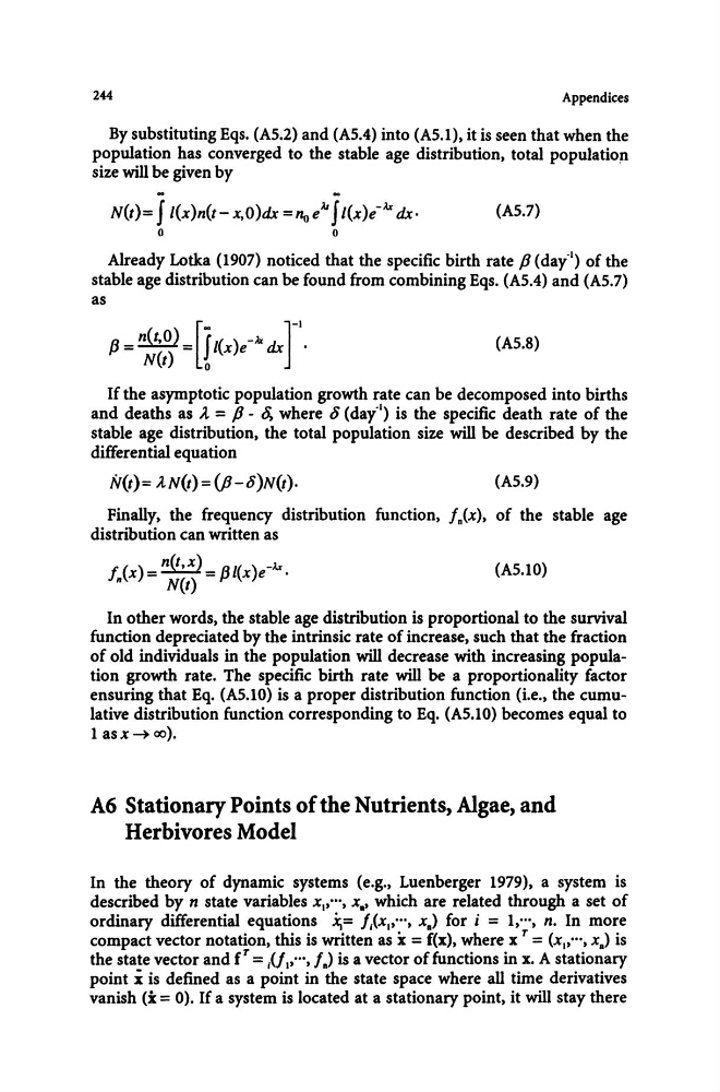
By substituting Eqs. (A5.2) and (A5.4) into (A5.1). it is seen that when the
population has converged to the stable age distribution. total populatio~
size will be given by
-
..
N(t)= J l(x)n(t- x,O)dx ="0 i' J l(x)e-"" dx·
(A5.7)
o
0
Already Lotka (1907) noticed that the specific birth rate P (day"l) of the
stable age distribution can be found from combining Eqs. (A5.4) and (A5.7)
as
{3 = n(t,O) = [Jool(x)e-.w dx]-I.
N(t)
0
(A5.8)
If the asymptotic population growth rate can be decomposed into births
and deaths as A. = P - ~ where 8 (day"l) is the specific death rate of the
stable age distribution. the total population size will be described by the
differential equation
N(t)= ).,N(t) = (p -8)N(t).
(A5.9)
Finally. the frequency distribution function. f.(x). of the stable age
distnoution can written as
f. (x) = n(t, x) = {31(x)e-"".
"
N(t)
(A5.10)
In other words. the stable age distribution is proportional to the survival
function depreciated by the intrinsic rate of increase. such that the fraction
of old individuals in the population will decrease with increasing population growth rate. The specific birth rate will be a proportionality factor
ensuring that Eq. (A5.10) is a proper distribution function (i.e .• the cumulative distribution function corresponding to Eq. (A5.10) becomes equal to
1 asx~ 00).
A6 Stationary Points of the Nutrients, Algae, and
Herbivores Model
In the theory of dynamic systems (e.g .• Luenberger 1979). a system is
described by n state variables Xl .. ••• x.' which are related through a set of
ordinary differential equations .ij= f,(xl .. ••• x.) for i = 1 .. ··• n. In more
compact vector notation. this is written as x = f(x). where x T = (Xl .. ••• x.) is
the state vector and fT = l(fl'···. f.) is a vector of functions in L A stationary
point i is defined as a point in the state space where all time derivatives
vanish (x = 0). If a system is located at a stationary point, it will stay there
Appendices
By substituting Eqs. (A5.2) and (A5.4) into (A5.1). it is seen that when the
population has converged to the stable age distribution. total populatio~
size will be given by
-
..
N(t)= J l(x)n(t- x,O)dx ="0 i' J l(x)e-"" dx·
(A5.7)
o
0
Already Lotka (1907) noticed that the specific birth rate P (day"l) of the
stable age distribution can be found from combining Eqs. (A5.4) and (A5.7)
as
{3 = n(t,O) = [Jool(x)e-.w dx]-I.
N(t)
0
(A5.8)
If the asymptotic population growth rate can be decomposed into births
and deaths as A. = P - ~ where 8 (day"l) is the specific death rate of the
stable age distribution. the total population size will be described by the
differential equation
N(t)= ).,N(t) = (p -8)N(t).
(A5.9)
Finally. the frequency distribution function. f.(x). of the stable age
distnoution can written as
f. (x) = n(t, x) = {31(x)e-"".
"
N(t)
(A5.10)
In other words. the stable age distribution is proportional to the survival
function depreciated by the intrinsic rate of increase. such that the fraction
of old individuals in the population will decrease with increasing population growth rate. The specific birth rate will be a proportionality factor
ensuring that Eq. (A5.10) is a proper distribution function (i.e .• the cumulative distribution function corresponding to Eq. (A5.10) becomes equal to
1 asx~ 00).
A6 Stationary Points of the Nutrients, Algae, and
Herbivores Model
In the theory of dynamic systems (e.g .• Luenberger 1979). a system is
described by n state variables Xl .. ••• x.' which are related through a set of
ordinary differential equations .ij= f,(xl .. ••• x.) for i = 1 .. ··• n. In more
compact vector notation. this is written as x = f(x). where x T = (Xl .. ••• x.) is
the state vector and fT = l(fl'···. f.) is a vector of functions in L A stationary
point i is defined as a point in the state space where all time derivatives
vanish (x = 0). If a system is located at a stationary point, it will stay there