

240
Appendices
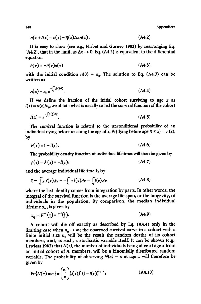
n(x +/u)= n(x)-l1(x)~n(x).
(A4.2)
It is easy to show (see e.g., Nisbet and Gurney 1982) by rearranging Eq.
(A4.2), that in the limit, as l\x ~ 0, Eq. (A4.2) is equivalent to the differential
equation
n{x) = -1](x)n{x)
(A4.3)
with the initial condition n(O) = no' The solution to Eq. (A4.3) can be
written as
(A4.4)
If we define the fraction of the initial cohort surviving to age x as
l(x) = n(x)/flo, we obtain what is usually called the survival function of the cohort
l(x) = e -J:,,(~)d~.
(A4.5)
The survival function is related to the unconditional probability of an
individual dying before reaching the age of x, Pr{dying before age X ~ x} = F(x),
by
F(x) = I-l(x).
(A4.6)
The probability density function of individual lifetimes will then be given by
f(x) = P{x)= -i{x),
(A4.7)
and the average individual lifetime X, by
x = [x f(x)dt = - [ xi(x)dt = [l(x)dt,
(A4.8)
where the last identity comes from integration by parts. In other words, the
integral of the survival function is the average life span, or the longevity, of
individuals in the population. By comparison, the median individual
lifetime x~, is given by
(A4.9)
A cohort will die off exactly as described by Eq. (A4.4) only in the
limiting case when no ~ 00; the observed survival curve in a cohort with a
finite initial size no will be the result the random deaths of its cohort
members, and, as such, a stochastic variable itself. It can be shown (e.g.,
Lawless 1982) that N(x), the number of individuals being alive at age x from
an initial cohort of no members, will be a binomially distributed random
variable. The probability of observing N(x) = n at age x will therefore be
given by
Pr{N(x) = n}= ( ~ ) (t(x»)" {I _l(x»)"o-n ,
(A4.10)
Appendices
n(x +/u)= n(x)-l1(x)~n(x).
(A4.2)
It is easy to show (see e.g., Nisbet and Gurney 1982) by rearranging Eq.
(A4.2), that in the limit, as l\x ~ 0, Eq. (A4.2) is equivalent to the differential
equation
n{x) = -1](x)n{x)
(A4.3)
with the initial condition n(O) = no' The solution to Eq. (A4.3) can be
written as
(A4.4)
If we define the fraction of the initial cohort surviving to age x as
l(x) = n(x)/flo, we obtain what is usually called the survival function of the cohort
l(x) = e -J:,,(~)d~.
(A4.5)
The survival function is related to the unconditional probability of an
individual dying before reaching the age of x, Pr{dying before age X ~ x} = F(x),
by
F(x) = I-l(x).
(A4.6)
The probability density function of individual lifetimes will then be given by
f(x) = P{x)= -i{x),
(A4.7)
and the average individual lifetime X, by
x = [x f(x)dt = - [ xi(x)dt = [l(x)dt,
(A4.8)
where the last identity comes from integration by parts. In other words, the
integral of the survival function is the average life span, or the longevity, of
individuals in the population. By comparison, the median individual
lifetime x~, is given by
(A4.9)
A cohort will die off exactly as described by Eq. (A4.4) only in the
limiting case when no ~ 00; the observed survival curve in a cohort with a
finite initial size no will be the result the random deaths of its cohort
members, and, as such, a stochastic variable itself. It can be shown (e.g.,
Lawless 1982) that N(x), the number of individuals being alive at age x from
an initial cohort of no members, will be a binomially distributed random
variable. The probability of observing N(x) = n at age x will therefore be
given by
Pr{N(x) = n}= ( ~ ) (t(x»)" {I _l(x»)"o-n ,
(A4.10)