

The fate of Zooplankton Egesta: Carbon Cycling and Chaos
199
0.8
-..
-;'
I-<
CO
..... 0.6
....
- ,.......,
U
b.O
e 0.4
'--'
' - '
c
0
.c
~ 0.2
u
'" 0
0
~
~
\
~ ~ ~ ~
~
~~
~ ~
~
V \. \ w, \\ tc \ \v ~ ~ \ ~ V,
J
0.0
o
100
200
300
Time Cd)
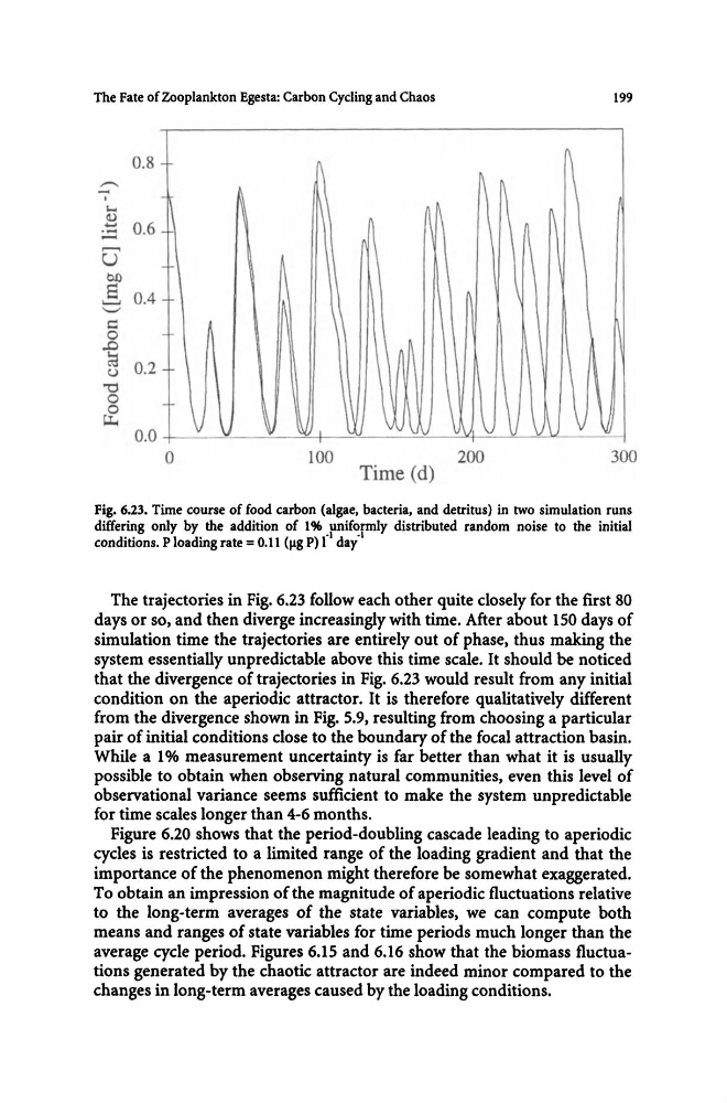
fig. 6.23. Time course of food carbon (algae, bacteria, and detritus) in two simulation runs
differing only by the addition of 1% uniformly distributed random noise to the initial
conditions. P loading rate = 0.11 (J.lg P) 1" day"
The trajectories in Fig. 6.23 follow each other quite closely for the first 80
days or so, and then diverge increasingly with time. After about 150 days of
simulation time the trajectories are entirely out of phase, thus making the
system essentially unpredictable above this time scale. It should be noticed
that the divergence of trajectories in Fig. 6.23 would result from any initial
condition on the aperiodic attractor. It is therefore qualitatively different
from the divergence shown in Fig. 5.9, resulting from choosing a particular
pair of initial conditions close to the boundary of the focal attraction basin.
While a 1 % measurement uncertainty is far better than what it is usually
possible to obtain when observing natural communities, even this level of
observational variance seems sufficient to make the system unpredictable
for time scales longer than 4-6 months.
Figure 6.20 shows that the period-doubling cascade leading to aperiodic
cycles is restricted to a limited range of the loading gradient and that the
importance of the phenomenon might therefore be somewhat exaggerated.
To obtain an impression of the magnitude of aperiodic fluctuations relative
to the long-term averages of the state variables, we can compute both
means and ranges of state variables for time periods much longer than the
average cycle period. Figures 6.15 and 6.16 show that the biomass fluctuations generated by the chaotic attractor are indeed minor compared to the
changes in long-term averages caused by the loading conditions.
199
0.8
-..
-;'
I-<
CO
..... 0.6
....
- ,.......,
U
b.O
e 0.4
'--'
' - '
c
0
.c
~ 0.2
u
'" 0
0
~
~
\
~ ~ ~ ~
~
~~
~ ~
~
V \. \ w, \\ tc \ \v ~ ~ \ ~ V,
J
0.0
o
100
200
300
Time Cd)
fig. 6.23. Time course of food carbon (algae, bacteria, and detritus) in two simulation runs
differing only by the addition of 1% uniformly distributed random noise to the initial
conditions. P loading rate = 0.11 (J.lg P) 1" day"
The trajectories in Fig. 6.23 follow each other quite closely for the first 80
days or so, and then diverge increasingly with time. After about 150 days of
simulation time the trajectories are entirely out of phase, thus making the
system essentially unpredictable above this time scale. It should be noticed
that the divergence of trajectories in Fig. 6.23 would result from any initial
condition on the aperiodic attractor. It is therefore qualitatively different
from the divergence shown in Fig. 5.9, resulting from choosing a particular
pair of initial conditions close to the boundary of the focal attraction basin.
While a 1 % measurement uncertainty is far better than what it is usually
possible to obtain when observing natural communities, even this level of
observational variance seems sufficient to make the system unpredictable
for time scales longer than 4-6 months.
Figure 6.20 shows that the period-doubling cascade leading to aperiodic
cycles is restricted to a limited range of the loading gradient and that the
importance of the phenomenon might therefore be somewhat exaggerated.
To obtain an impression of the magnitude of aperiodic fluctuations relative
to the long-term averages of the state variables, we can compute both
means and ranges of state variables for time periods much longer than the
average cycle period. Figures 6.15 and 6.16 show that the biomass fluctuations generated by the chaotic attractor are indeed minor compared to the
changes in long-term averages caused by the loading conditions.