

Individual Mortality and Population Losses
99
1.0 """1<"""--------------------,
l(x)
0.8
btl
c:
.... > 0.6
.... >
~
v.l
c:
0 0.4
'.:;J
u
(OJ
~
0.2
0.0 -I-_~ __ _+_-----1_+--===:::::::::~
o
20
40
60
Age (d)
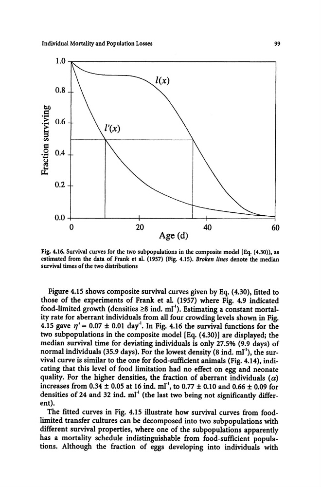
Fig. 4.16. Survival curves for the two subpopulations in the composite model [Eq. (4.30». as
estimated from the data of Frank et a1. (1957) (Fig. 4.15). Broken lines denote the median
survival times of the two distributions
Figure 4.15 shows composite survival curves given by Eq. (4.30), fitted to
those of the experiments of Frank et al. (1957) where Fig. 4.9 indicated
food-limited growth (densities ~8 indo mr l ). Estimating a constant mortality rate for aberrant individuals from all four crowding levels shown in Fig.
4.15 gave ,,' = 0.07 ± 0.01 day"l. In Fig. 4.16 the survival functions for the
two subpopulations in the composite model [Eq. (4.30)] are displayed; the
median survival time for deviating individuals is only 27.5% (9.9 days) of
normal individuals (35.9 days). For the lowest density (8 indo mr\ the survival curve is similar to the one for food-sufficient animals (Fig. 4.14), indicating that this level of food limitation had no effect on egg and neonate
quality. For the higher densities, the fraction of aberrant individuals (a)
increases from 0.34 ± 0.05 at 16 indo mr., to 0.77 ± 0.10 and 0.66 ± 0.09 for
densities of 24 and 32 indo mr l (the last two being not significantly different).
The fitted curves in Fig. 4.15 illustrate how survival curves from foodlimited transfer cultures can be decomposed into two subpopulations with
different survival properties, where one of the subpopulations apparently
has a mortality schedule indistinguishable from food-sufficient populations. Although the fraction of eggs developing into individuals with
99
1.0 """1<"""--------------------,
l(x)
0.8
btl
c:
.... > 0.6
.... >
~
v.l
c:
0 0.4
'.:;J
u
(OJ
~
0.2
0.0 -I-_~ __ _+_-----1_+--===:::::::::~
o
20
40
60
Age (d)
Fig. 4.16. Survival curves for the two subpopulations in the composite model [Eq. (4.30». as
estimated from the data of Frank et a1. (1957) (Fig. 4.15). Broken lines denote the median
survival times of the two distributions
Figure 4.15 shows composite survival curves given by Eq. (4.30), fitted to
those of the experiments of Frank et al. (1957) where Fig. 4.9 indicated
food-limited growth (densities ~8 indo mr l ). Estimating a constant mortality rate for aberrant individuals from all four crowding levels shown in Fig.
4.15 gave ,,' = 0.07 ± 0.01 day"l. In Fig. 4.16 the survival functions for the
two subpopulations in the composite model [Eq. (4.30)] are displayed; the
median survival time for deviating individuals is only 27.5% (9.9 days) of
normal individuals (35.9 days). For the lowest density (8 indo mr\ the survival curve is similar to the one for food-sufficient animals (Fig. 4.14), indicating that this level of food limitation had no effect on egg and neonate
quality. For the higher densities, the fraction of aberrant individuals (a)
increases from 0.34 ± 0.05 at 16 indo mr., to 0.77 ± 0.10 and 0.66 ± 0.09 for
densities of 24 and 32 indo mr l (the last two being not significantly different).
The fitted curves in Fig. 4.15 illustrate how survival curves from foodlimited transfer cultures can be decomposed into two subpopulations with
different survival properties, where one of the subpopulations apparently
has a mortality schedule indistinguishable from food-sufficient populations. Although the fraction of eggs developing into individuals with