

120
4. SIMULATING GROWTH AND FORM
for each phase until equilibrium, followed by a tracer step. To reduce the time
for the tracer distribution to attain an equilibrium, the tracer computation
uses two separate tracer distributions: a distribution for the case where the
flow is directed from left to right (tracer distribution A) and a distribution
for the case where the flow is directed from right to left (tracer distribution
B). If the flow at a certain time step is for example directed from left to
right, the results of a previous time step where the flow was directed from
left to right can be used to speed up the computation time. Tracer particles
are again released from the source plane, the lattice sites located at the xzplane at y = ymax for both phases, and tracer particles are absorbed by the
fluid nodes adjacent to obstacle nodes . The probability p that a new node
will be added to the aggregate is again computed using (4.18), using the
corresponding tracer distribution. After each growth step the flow direction
is reversed. The aggregation model for a bidirectional flow is summarized in
pseudo-code below:
initialize aggregate
initialize flow direction
initialize tracer distributions
do {
-if (flow from left to right) {
-compute flow velocities until equilibrium;
-compute tracer distribution A until equilibrium;
-select randomly with probability p (4 .18) , using tracer
distribution A, one of the growth candidates and
add it to the aggregate;}
-else(flow from right to left) {
-compute flow velocities until equilibrium;
-compute tracer distribution B until equilibrium;
-select randomly with probability p (4 .18), using tracer
distribution B, one of the growth candidates and
add it to the aggregate ;}
-reverse flow direction;
} until ready
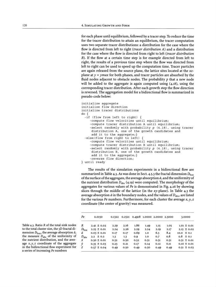
The results of the simulation experiments in a bidirectional flow are
summarized in Table4.3.Aswas done in Sect. 4.5.3 the fractal dimension Dt,ox
of the surface of the aggregate, the average absorption a, and the uniformity of
the nutrient distribution Dabs (4.19) were computed. The morphology of the
aggregates for various values of Pe is demonstrated in Fig. 4.26 by showing
slices through the middle of the lattice (in the xy-plane). In Table 4.3 the
average absorption ain the boundary nodes, and the values of Dabs, are listed
for the various Pe numbers. Furthermore, for each cluster the average x,y, z
coordinate (the center of gravity) was measured.
Pe
0.0150
0.1322 0 .2521 0·4918 1.0000 2.0000 2.50 0 0
3·0000
Table 4.3. Ratio R of the total sink nodes
R
2.41 ± 0 .02
2 .29
2.16
1.86
1·49
1.15
1.05
1.01 ± 0 .01
to the total cluster size, the 3D fractal di!\ox 2.25 ± 0 .01
2.24
2.26
2.29
2.24
2 .19
2.17
2.15 ± 0 .02
mension !\ox' the average absorption a, a
0.03 ± 0 .01
0.17
0.17
0.69
1.0
6 ·3
8.4
10.0 ± 0 .1
the measure Dabs of the uniformity of
Dabs 2.2 ± 0 .2
1·3
1.3
0·9
1.0
0 ·7
0.8
0.8 ± 0 .1
the nutrient distribution, and the averx
0.50 ± 0 .01
0·52
0·50
0·52
0·51
0 ·51
0·51
0.51 ± 0.01
age x, y, z coordinate of the aggregate s 0.35 ± 0 .03 0.23 0.21 0.17 0.14 0 .12 0.11 0.10 ± 0.01
in the bidirectional flow experiment for
Ii
0.57 ± 0 .04
0·49
0 ·50
0-49
0·50
0 ·49
0-49
0 .51 ± 0.03
a series of increasing Penumbers
4. SIMULATING GROWTH AND FORM
for each phase until equilibrium, followed by a tracer step. To reduce the time
for the tracer distribution to attain an equilibrium, the tracer computation
uses two separate tracer distributions: a distribution for the case where the
flow is directed from left to right (tracer distribution A) and a distribution
for the case where the flow is directed from right to left (tracer distribution
B). If the flow at a certain time step is for example directed from left to
right, the results of a previous time step where the flow was directed from
left to right can be used to speed up the computation time. Tracer particles
are again released from the source plane, the lattice sites located at the xzplane at y = ymax for both phases, and tracer particles are absorbed by the
fluid nodes adjacent to obstacle nodes . The probability p that a new node
will be added to the aggregate is again computed using (4.18), using the
corresponding tracer distribution. After each growth step the flow direction
is reversed. The aggregation model for a bidirectional flow is summarized in
pseudo-code below:
initialize aggregate
initialize flow direction
initialize tracer distributions
do {
-if (flow from left to right) {
-compute flow velocities until equilibrium;
-compute tracer distribution A until equilibrium;
-select randomly with probability p (4 .18) , using tracer
distribution A, one of the growth candidates and
add it to the aggregate;}
-else(flow from right to left) {
-compute flow velocities until equilibrium;
-compute tracer distribution B until equilibrium;
-select randomly with probability p (4 .18), using tracer
distribution B, one of the growth candidates and
add it to the aggregate ;}
-reverse flow direction;
} until ready
The results of the simulation experiments in a bidirectional flow are
summarized in Table4.3.Aswas done in Sect. 4.5.3 the fractal dimension Dt,ox
of the surface of the aggregate, the average absorption a, and the uniformity of
the nutrient distribution Dabs (4.19) were computed. The morphology of the
aggregates for various values of Pe is demonstrated in Fig. 4.26 by showing
slices through the middle of the lattice (in the xy-plane). In Table 4.3 the
average absorption ain the boundary nodes, and the values of Dabs, are listed
for the various Pe numbers. Furthermore, for each cluster the average x,y, z
coordinate (the center of gravity) was measured.
Pe
0.0150
0.1322 0 .2521 0·4918 1.0000 2.0000 2.50 0 0
3·0000
Table 4.3. Ratio R of the total sink nodes
R
2.41 ± 0 .02
2 .29
2.16
1.86
1·49
1.15
1.05
1.01 ± 0 .01
to the total cluster size, the 3D fractal di!\ox 2.25 ± 0 .01
2.24
2.26
2.29
2.24
2 .19
2.17
2.15 ± 0 .02
mension !\ox' the average absorption a, a
0.03 ± 0 .01
0.17
0.17
0.69
1.0
6 ·3
8.4
10.0 ± 0 .1
the measure Dabs of the uniformity of
Dabs 2.2 ± 0 .2
1·3
1.3
0·9
1.0
0 ·7
0.8
0.8 ± 0 .1
the nutrient distribution, and the averx
0.50 ± 0 .01
0·52
0·50
0·52
0·51
0 ·51
0·51
0.51 ± 0.01
age x, y, z coordinate of the aggregate s 0.35 ± 0 .03 0.23 0.21 0.17 0.14 0 .12 0.11 0.10 ± 0.01
in the bidirectional flow experiment for
Ii
0.57 ± 0 .04
0·49
0 ·50
0-49
0·50
0 ·49
0-49
0 .51 ± 0.03
a series of increasing Penumbers