

110
+
I
I.
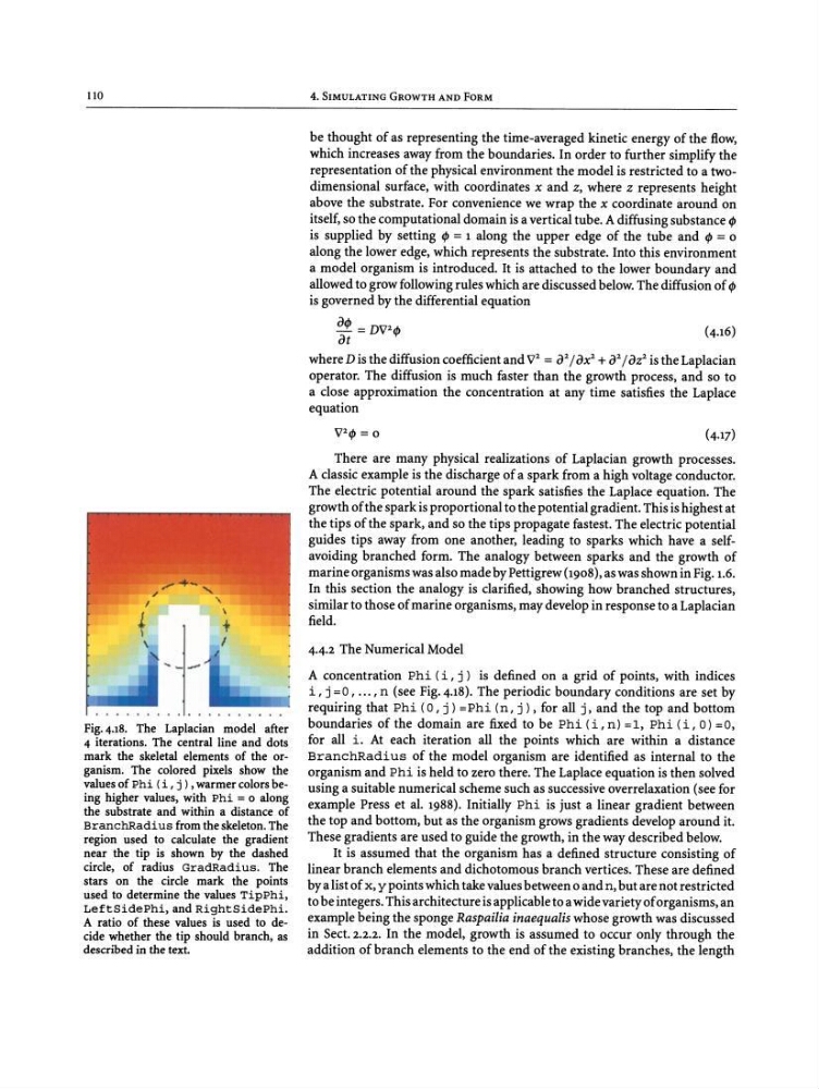
Fig. 4.18. The Laplacian model after
4 iterations. The central line and dots
mark the skeletal elements of the organism. The colored pixels show the
values of Phi (i , j ) , warmercolors being higher values, with Phi = 0 along
the substrate and within a distance of
BranchRadius fromtheskeleton. The
region used to calculate the gradient
near the tip is shown by the dashed
circle, of radius GradRadius. The
stars on the circle mark the points
used to determine the values TipPhi,
LeftSidePhi, and RightSidePhi.
A ratio of these values is used to decide whether the tip should branch, as
described in the text.
4 . SIMULATING GROWTH AN D FORM
be thought of as representing the time-averaged kinetic energy of the flow,
which increases away from the boundaries. In order to further simplify the
representation of the physical environment the model is restricted to a twodimensional surface, with coordinates x and z, where z represents height
above the substrate. For convenience we wrap the x coordinate around on
itself, so the computational domain is a vertical tube. A diffusing substance
a model organism is introduced. It is attached to the lower boundary and
allowed to grow following rules which are discussed below. The diffusion of
alP = DV2
at
where D is the diffusion coefficient and v
2 = a 2 / ax 2 + a 2 / az 2 is the Laplacian
operator. The diffusion is much faster than the growth process, and so to
a close approximation the concentration at any time satisfies the Laplace
equation
V2 There are many physical realizations of Laplacian growth processes.
A classic example is the discharge of a spark from a high voltage conductor.
The electric potential around the spark satisfies the Laplace equation. The
growth of the spark is proportional to the potential gradient. This is highest at
the tips of the spark, and so the tips propagate fastest. The electric potential
guides tips away from one another, leading to sparks which have a selfavoiding branched form. The analogy between sparks and the growth of
marine organisms was also made by Pettigrew (1908), as was shown in Fig. 1.6.
In this section the analogy is clarified, showing how branched structures,
similar to those of marine organisms, may develop in response to a Laplacian
field.
4.4.2 The Numerical Model
A concentration Phi (i, j) is defined on a grid of points, with indices
i, j =0, ... , n (see Fig. 4.18). The periodic boundary conditions are set by
requiring that Ph i (0 , j ) = Phi (n, j ) , for all j, and the top and bottom
boundaries of the domain are fixed to be Phi ( i , n) = 1, Phi (i , 0) = 0,
for all i. At each iteration all the points which are within a distance
BranchRadius of the model organism are identified as internal to the
organism and Phi is held to zero there. The Laplace equation is then solved
using a suitable numerical scheme such as successive overrelaxation (see for
example Press et al. 1988). Initially Phi is just a linear gradient between
the top and bottom, but as the organism grows gradients develop around it.
These gradients are used to guide the growth, in the way described below.
It is assumed that the organism has a defined structure consisting of
linear branch elements and dichotomous branch vertices. These are defined
by a list of x, y points which take values between 0 and n, but are not restricted
to be integers. This architecture is applicable to a wide variety of organisms, an
example being the sponge Raspailia inaequalis whose growth was discussed
in Sect. 2.2.2. In the model, growth is assumed to occur only through the
addition of branch elements to the end of the existing branches, the length
+
I
I.
Fig. 4.18. The Laplacian model after
4 iterations. The central line and dots
mark the skeletal elements of the organism. The colored pixels show the
values of Phi (i , j ) , warmercolors being higher values, with Phi = 0 along
the substrate and within a distance of
BranchRadius fromtheskeleton. The
region used to calculate the gradient
near the tip is shown by the dashed
circle, of radius GradRadius. The
stars on the circle mark the points
used to determine the values TipPhi,
LeftSidePhi, and RightSidePhi.
A ratio of these values is used to decide whether the tip should branch, as
described in the text.
4 . SIMULATING GROWTH AN D FORM
be thought of as representing the time-averaged kinetic energy of the flow,
which increases away from the boundaries. In order to further simplify the
representation of the physical environment the model is restricted to a twodimensional surface, with coordinates x and z, where z represents height
above the substrate. For convenience we wrap the x coordinate around on
itself, so the computational domain is a vertical tube. A diffusing substance
a model organism is introduced. It is attached to the lower boundary and
allowed to grow following rules which are discussed below. The diffusion of
alP = DV2
at
where D is the diffusion coefficient and v
2 = a 2 / ax 2 + a 2 / az 2 is the Laplacian
operator. The diffusion is much faster than the growth process, and so to
a close approximation the concentration at any time satisfies the Laplace
equation
V2 There are many physical realizations of Laplacian growth processes.
A classic example is the discharge of a spark from a high voltage conductor.
The electric potential around the spark satisfies the Laplace equation. The
growth of the spark is proportional to the potential gradient. This is highest at
the tips of the spark, and so the tips propagate fastest. The electric potential
guides tips away from one another, leading to sparks which have a selfavoiding branched form. The analogy between sparks and the growth of
marine organisms was also made by Pettigrew (1908), as was shown in Fig. 1.6.
In this section the analogy is clarified, showing how branched structures,
similar to those of marine organisms, may develop in response to a Laplacian
field.
4.4.2 The Numerical Model
A concentration Phi (i, j) is defined on a grid of points, with indices
i, j =0, ... , n (see Fig. 4.18). The periodic boundary conditions are set by
requiring that Ph i (0 , j ) = Phi (n, j ) , for all j, and the top and bottom
boundaries of the domain are fixed to be Phi ( i , n) = 1, Phi (i , 0) = 0,
for all i. At each iteration all the points which are within a distance
BranchRadius of the model organism are identified as internal to the
organism and Phi is held to zero there. The Laplace equation is then solved
using a suitable numerical scheme such as successive overrelaxation (see for
example Press et al. 1988). Initially Phi is just a linear gradient between
the top and bottom, but as the organism grows gradients develop around it.
These gradients are used to guide the growth, in the way described below.
It is assumed that the organism has a defined structure consisting of
linear branch elements and dichotomous branch vertices. These are defined
by a list of x, y points which take values between 0 and n, but are not restricted
to be integers. This architecture is applicable to a wide variety of organisms, an
example being the sponge Raspailia inaequalis whose growth was discussed
in Sect. 2.2.2. In the model, growth is assumed to occur only through the
addition of branch elements to the end of the existing branches, the length