

628
Susan S. Bell, Mark S. Fonseca, and Nathaniel B. Stafford
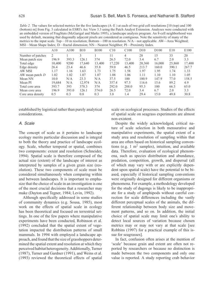
Table 2. The values for selected metrics for the five landscapes (A–E ) at each of two grid cell resolutions [10 (top) and 100
(bottom) m] from Fig. 3 calculated in ESRI’s Arc View 3.3 using the Patch Analyst Extension. Analyses were conducted with
an embedded version of FragStats (McGarigal and Marks 1995), a landscape analysis program. An 8-cell neighborhood was
used by default, meaning that diagonally adjacent pixels are considered as contiguous. Note the sensitivity of many of the
metrics to the input scale. Top—10 m resolution; Bottom—100 m resolution. N/A—not applicable. AW—Area Weighted;
MSI—Mean Shape Index; D—fractal dimension; NN—Nearest Neighbor; PI—Proximity Index.
A10
A100
B10
B100
C10
C100
D10
D100
E10
E100
Number of patches
2
1
3
1
11
4
28
15
33
20
Mean patch size
196.9
393.3
126.1
374
26.5
72.0
3.4
6.7
2.0
3.3
Total edge
10,400
9200
17,640
13,400
17,220
13,400
20,360
16,000
25,860
17,400
Edge density
26.4
23.4
46.6
35.8
59.0
46.5
213.7
160.0
390.1
267.7
AW MSI
1.17
1.16
1.63
1.73
1.75
1.58
1.97
1.95
1.74
1.33
AW mean patch D
1.02
1.02
1.07
1.07
1.08
1.06
1.11
1.10
1.10
1.05
Mean NN
10.0
N/A
23.3
N/A
37.5
100
100.9
147.9
77.0
158.5
Mean PI
19,684
N/A
12,974
N/A
357.4
97.5
116.6
15.6
89.2
4.9
Total core area
393.7
393
378.3
374
292.0
288.0
95.3
100
66.3
65.0
Mean core area
196.9
393.0
126.1
374.0
26.5
72.0
3.4
6.7
2.0
3.3
Core area density
0.5
0.3
0.8
0.3
3.8
1.4
29.4
15.0
49.8
30.8
established by logistical rather than purely analytical
considerations.
A. Scale
The concept of scale as it pertains to landscape
ecology merits particular discussion and is integral
to both the theory and practice of landscape ecology. Scale, whether temporal or spatial, combines
two components: extent and resolution (Schneider,
1994). Spatial scale is therefore composed of the
actual size (extent) of the landscape of interest as
interpreted by samples of a given grain size (resolution). These two components of scale must be
considered simultaneously when comparing within
and between landscapes. It is important to emphasize that the choice of scale in an investigation is one
of the most crucial decisions that a researcher may
make (Dayton and Tegner, 1984; Levin, 1992).
Although specifically addressed in some studies
of community dynamics (e.g. Sousa, 1985), most
work on the effects of spatial scale in ecology
has been theoretical and focused on terrestrial settings. In one of the few papers where manipulative
experiments have been conducted, Robinson et al.
(1992) concluded that the spatial extent of vegetation impacted the distribution patterns of small
mammals. In 1994 with employed a landscape approach, and found that the size of grasshoppers determined the spatial extent and resolution at which they
perceived habitat heterogeneity. Additionally, Turner
(1987), Turner and Gardner (1991), and Weins et al.
(1993) reviewed the theoretical effects of spatial
scale on ecological processes. Studies of the effects
of spatial scale on seagrass experiments are almost
non-existent.
Despite the widely acknowledged, critical nature of scale selection in both mensurative and
manipulative experiments, the spatial extent of a
study area and resolution of sampling within that
area are often based on historical sampling conventions (e.g. 1 m
2 samples), intuition, and available
data. Therefore, evaluation of ecological phenomena, such as species distribution and abundance,
predation, competition, growth, and dispersal (all
of which may vary with or are explicitly dependent upon spatial scale) have the potential to be biased, especially if historical sampling conventions
were originally designed for different organisms or
phenomena. For example, a methodology developed
for the study of dugongs is likely to be inappropriate for a study of amphipods without careful correction for scale differences including the vastly
different perceptual scales of the animals, the different relationship between body size and movement patterns, and so on. In addition, the initial
choice of spatial scale may limit one’s ability to
detect local sources of variation because chosen
metrics may or may not vary at that scale [see
Robbins (1997) for a practical example of this issue for seagrasses].
In fact, confusion often arises at the mention of
‘scale’ because grain and extent are often not reported by researchers or because no distinction is
made between the two components and only one
value is reported. A study reporting crab behavior