

the head of the bay, but friction will keep that tide range
much smaller than it would be without friction.
(Mathematical formulas representing the effects described
above are derived in Parker, 2007).
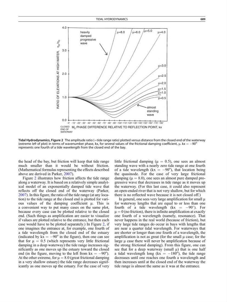
Figure 2 illustrates how friction affects the tide range
along a waterway. It is based on a relatively simple analytical model of an exponentially damped tide wave that
reflects off the closed end of the waterway (Parker,
2007). In this figure, the ratio of the tide range (at any location) to the tide range at the closed end is plotted for various values of the damping coefficient m. This is
a convenient way to put many cases on the same plot,
because every case can be plotted relative to the closed
end. (Such things as amplification are easier to visualize
if values are plotted relative to the entrance, but then each
case would have to be plotted separately.) In Figure 2, if
one imagines the entrance at, for example, one fourth of
a tide wavelength from the closed end of the estuary
(indicated by kx ¼ À90
o in the figure), then one can see
that for m ¼ 0.5 (which represents very little frictional
damping in a deep waterway) the tide range increases significantly as one moves up the estuary toward the closed
end (in the figure, moving to the left from kx ¼ À90
o
).
At the other extreme, for m ¼ 8.0 (great frictional damping
in a very shallow estuary) the tide range decreases significantly as one moves up the estuary. For the case of very
little frictional damping (m ¼ 0.5), one sees an almost
standing wave with a nearly zero tide range at one fourth
of a tide wavelength (kx ¼ À90
o
), that location being
the quasinode. For the case of very large frictional
damping (m ¼ 8.0), one sees an almost pure damped progressive wave that decreases in tide range as it moves up
the waterway. (For this last case, it could also represent
an open-ended river that is not very shallow, but for which
there is no reflected wave because it is not closed off.)
In general, one sees very large amplification for small m
for waterway lengths that are equal to or less than one
fourth of a tide wavelength (kx ¼ À90
). For
m ¼ 0 (no friction), there is infinite amplification at exactly
one fourth of a wavelength (namely, resonance). That
never happens in the real world (because of friction), but
very large tide ranges do occur in bays with lengths that
are near a quarter tidal wavelength. For waterways that
are shorter or longer than one fourth of a wavelength, the
amplification is not as great (for the small m case; for the
large m case there will never be amplification because of
the strong frictional damping). From this figure, one can
see that for a deep waterway (small m) that is one half
a tidal wavelength long (kx ¼ À180
o ), the tide range
decreases until one reaches one fourth a wavelength and
then increases until at the closed end of the waterway the
tide range is almost the same as it was at the entrance.
4.0
heavily
damped
progressive
wave
μ=8.0
μ=6.0 μ=5.0
μ=4.0
μ=3.0
μ=2.5
μ=2.0
μ=1.5
μ=1.0
μ=0.5
3.0
2.0
1.0
RATIO OF ELEVATIONS AT HIGH WATER,
η
H /η
0
M 2 PHASE DIFFERENCE RELATIVE TO REFLECTION POINT, kx
0.0
CLOSED
END OF
WATERWAY
−0Њ −10Њ −20Њ −30Њ −40Њ −50Њ −60Њ −70Њ −80Њ −90Њ −100Њ−110Њ−120Њ−130Њ−140Њ−150Њ−160Њ−170Њ−180Њ
almost
standing
wave
Tidal Hydrodynamics, Figure 2 The amplitude ratio (¼tide range ratio) plotted versus distance from the closed end of the waterway
(extreme left of plot) in terms of wavenumber phase, kx, for several values of the frictional damping coefficient, m. kx ¼ À90
o
represents one fourth of a tide wavelength from the closed end of the bay.
TIDAL HYDRODYNAMICS
689