

Once established, calibration curves can be used, for
example, to calculate sediment fluxes over time from
volume changes determined for specific areas within
estuaries, either by repeated multibeam bathymetric surveys (in subtidal settings) or precision leveling
(in intertidal settings). The procedure for converting volumetric changes into sediment masses, either positive
(gain) or negative (loss), is illustrated in the flow chart
of Figure 7a (cf. Bartholomä et al., 2000). Besides the
total sediment flux, the flux of the sand and mud fractions
can also be determined if the contributions of these to the
total sediment are known. This also applies to any other
known sediment component, as illustrated for standing
stocks in Figure 7b and fluxes of POC in Figure 7c
(cf. Delafontaine et al., 2000). The same general procedures can be applied to other organic or inorganic
substances, provided their contents are known.
Potential pitfalls
As pointed out above, contents (masses per unit mass)
and concentrations (masses per unit volume) are
often confused or even understood to mean the same
thing. This can lead to serious errors where parameters
of the one, e.g., species numbers per square meter
(a measure of concentration), are directly related to
parameters of the other, e.g., percent organic matter
(a measure of content), over a range of sand–mud mixtures. By doing this, it is overlooked that the dimensional
incompatibility will cause misrepresentations and faulty
assessments.
To highlight the nature of this problem, a mud
concentration model is contrasted with a mud content
model for a sand–mud gradient in the Wadden Sea
(Figure 8). It can be viewed as representing either
a transect or a vertical sediment column (core) ranging in
composition from pure sand (yellow boxes at bottom) to
pure mud (dark blue boxes at top). Due to the progressive
decrease in bulk density with increasing mud content, the
sediment mass in a unit volume of sediment (e.g., 1 l or
1 dm
3 ) decreases from about 1.5 g cm
À3 in sand to about
0.3 g cm
À3 in mud (mud concentration model). Any other
sediment component (e.g., organic matter, POC, heavy
metals, toxic substances) would decrease proportionally
and, in this example, follow the trend defined by the blue
line representing the mud concentration (graph on the
right). Clearly, when relating parameters such as
species numbers per m
2 to the potentially available food,
the concentration of organic matter or POC has to be
chosen for meaningful comparison. If organic matter or
POC contents were used instead, as is commonly observed
in the literature, one would be comparing the species
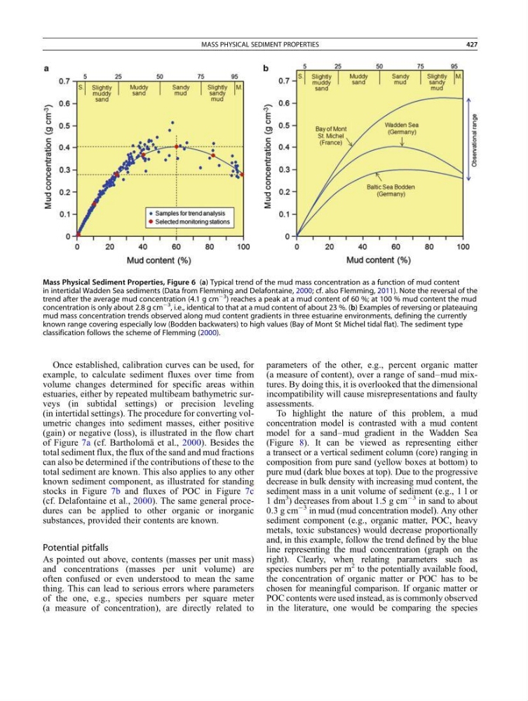
Mass Physical Sediment Properties, Figure 6 (a) Typical trend of the mud mass concentration as a function of mud content
in intertidal Wadden Sea sediments (Data from Flemming and Delafontaine, 2000; cf. also Flemming, 2011). Note the reversal of the
trend after the average mud concentration (4.1 g cm
À3 ) reaches a peak at a mud content of 60 %; at 100 % mud content the mud
concentration is only about 2.8 g cm
À3 , i.e., identical to that at a mud content of about 23 %. (b) Examples of reversing or plateauing
mud mass concentration trends observed along mud content gradients in three estuarine environments, defining the currently
known range covering especially low (Bodden backwaters) to high values (Bay of Mont St Michel tidal flat). The sediment type
classification follows the scheme of Flemming (2000).
MASS PHYSICAL SEDIMENT PROPERTIES
427
example, to calculate sediment fluxes over time from
volume changes determined for specific areas within
estuaries, either by repeated multibeam bathymetric surveys (in subtidal settings) or precision leveling
(in intertidal settings). The procedure for converting volumetric changes into sediment masses, either positive
(gain) or negative (loss), is illustrated in the flow chart
of Figure 7a (cf. Bartholomä et al., 2000). Besides the
total sediment flux, the flux of the sand and mud fractions
can also be determined if the contributions of these to the
total sediment are known. This also applies to any other
known sediment component, as illustrated for standing
stocks in Figure 7b and fluxes of POC in Figure 7c
(cf. Delafontaine et al., 2000). The same general procedures can be applied to other organic or inorganic
substances, provided their contents are known.
Potential pitfalls
As pointed out above, contents (masses per unit mass)
and concentrations (masses per unit volume) are
often confused or even understood to mean the same
thing. This can lead to serious errors where parameters
of the one, e.g., species numbers per square meter
(a measure of concentration), are directly related to
parameters of the other, e.g., percent organic matter
(a measure of content), over a range of sand–mud mixtures. By doing this, it is overlooked that the dimensional
incompatibility will cause misrepresentations and faulty
assessments.
To highlight the nature of this problem, a mud
concentration model is contrasted with a mud content
model for a sand–mud gradient in the Wadden Sea
(Figure 8). It can be viewed as representing either
a transect or a vertical sediment column (core) ranging in
composition from pure sand (yellow boxes at bottom) to
pure mud (dark blue boxes at top). Due to the progressive
decrease in bulk density with increasing mud content, the
sediment mass in a unit volume of sediment (e.g., 1 l or
1 dm
3 ) decreases from about 1.5 g cm
À3 in sand to about
0.3 g cm
À3 in mud (mud concentration model). Any other
sediment component (e.g., organic matter, POC, heavy
metals, toxic substances) would decrease proportionally
and, in this example, follow the trend defined by the blue
line representing the mud concentration (graph on the
right). Clearly, when relating parameters such as
species numbers per m
2 to the potentially available food,
the concentration of organic matter or POC has to be
chosen for meaningful comparison. If organic matter or
POC contents were used instead, as is commonly observed
in the literature, one would be comparing the species
Mass Physical Sediment Properties, Figure 6 (a) Typical trend of the mud mass concentration as a function of mud content
in intertidal Wadden Sea sediments (Data from Flemming and Delafontaine, 2000; cf. also Flemming, 2011). Note the reversal of the
trend after the average mud concentration (4.1 g cm
À3 ) reaches a peak at a mud content of 60 %; at 100 % mud content the mud
concentration is only about 2.8 g cm
À3 , i.e., identical to that at a mud content of about 23 %. (b) Examples of reversing or plateauing
mud mass concentration trends observed along mud content gradients in three estuarine environments, defining the currently
known range covering especially low (Bodden backwaters) to high values (Bay of Mont St Michel tidal flat). The sediment type
classification follows the scheme of Flemming (2000).
MASS PHYSICAL SEDIMENT PROPERTIES
427