

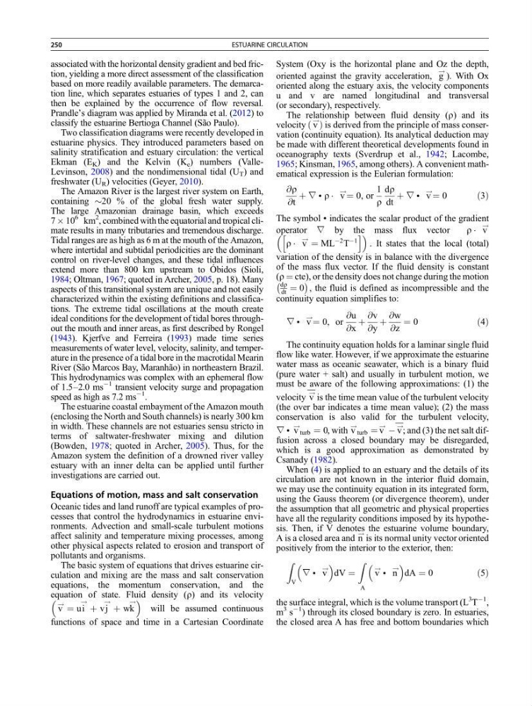
associated with the horizontal density gradient and bed friction, yielding a more direct assessment of the classification
based on more readily available parameters. The demarcation line, which separates estuaries of types 1 and 2, can
then be explained by the occurrence of flow reversal.
Prandle’s diagram was applied by Miranda et al. (2012) to
classify the estuarine Bertioga Channel (São Paulo).
Two classification diagrams were recently developed in
estuarine physics. They introduced parameters based on
salinity stratification and estuary circulation: the vertical
Ekman (E K ) and the Kelvin (K e ) numbers (ValleLevinson, 2008) and the nondimensional tidal (U T ) and
freshwater (U R ) velocities (Geyer, 2010).
The Amazon River is the largest river system on Earth,
containing $20 % of the global fresh water supply.
The large Amazonian drainage basin, which exceeds
7 Â 10
6 km
2
, combined with the equatorial and tropical climate results in many tributaries and tremendous discharge.
Tidal ranges are as high as 6 m at the mouth of the Amazon,
where intertidal and subtidal periodicities are the dominant
control on river-level changes, and these tidal influences
extend more than 800 km upstream to Óbidos (Sioli,
1984; Oltman, 1967; quoted in Archer, 2005, p. 18). Many
aspects of this transitional system are unique and not easily
characterized within the existing definitions and classifications. The extreme tidal oscillations at the mouth create
ideal conditions for the development of tidal bores throughout the mouth and inner areas, as first described by Rongel
(1943). Kjerfve and Ferreira (1993) made time series
measurements of water level, velocity, salinity, and temperature in the presence of a tidal bore in the macrotidal Mearin
River (São Marcos Bay, Maranhão) in northeastern Brazil.
This hydrodynamics was complex with an ephemeral flow
of 1.5–2.0 ms
À1 transient velocity surge and propagation
speed as high as 7.2 ms
À1
.
The estuarine coastal embayment of the Amazon mouth
(enclosing the North and South channels) is nearly 300 km
in width. These channels are not estuaries sensu stricto in
terms of saltwater-freshwater mixing and dilution
(Bowden, 1978; quoted in Archer, 2005). Thus, for the
Amazon system the definition of a drowned river valley
estuary with an inner delta can be applied until further
investigations are carried out.
Equations of motion, mass and salt conservation
Oceanic tides and land runoff are typical examples of processes that control the hydrodynamics in estuarine environments. Advection and small-scale turbulent motions
affect salinity and temperature mixing processes, among
other physical aspects related to erosion and transport of
pollutants and organisms.
The basic system of equations that drives estuarine circulation and mixing are the mass and salt conservation
equations, the momentum conservation, and the
equation of state. Fluid density (r) and its velocity
v
! ¼ ui
! þ vj
! þ wk
!
will be assumed continuous
functions of space and time in a Cartesian Coordinate
System (Oxy is the horizontal plane and Oz the depth,
oriented against the gravity acceleration, g
! ). With Ox
oriented along the estuary axis, the velocity components
u and v are named longitudinal and transversal
(or secondary), respectively.
The relationship between fluid density (r) and its
velocity ð v
!
Þ is derived from the principle of mass conservation (continuity equation). Its analytical deduction may
be made with different theoretical developments found in
oceanography texts (Sverdrup et al., 1942; Lacombe,
1965; Kinsman, 1965, among others). A convenient mathematical expression is the Eulerian formulation:
@r
@t
þ ∇ • r Á v
!
¼ 0, or
1
r
dr
dt
þ ∇ • v
!
¼ 0
ð3Þ
The symbol • indicates the scalar product of the gradient
operator ∇ by the mass flux vector
r Á v
!
r Á v
! ¼ ML
À2 T
À1
h
i
. It states that the local (total)
variation of the density is in balance with the divergence
of the mass flux vector. If the fluid density is constant
(r ¼ cte), or the density does not change during the motion
dr
dt ¼ 0
À
Á
, the fluid is defined as incompressible and the
continuity equation simplifies to:
∇ • v
!
¼ 0, or
@u
@x
þ
@v
@y
þ
@w
@z
¼ 0
ð4Þ
The continuity equation holds for a laminar single fluid
flow like water. However, if we approximate the estuarine
water mass as oceanic seawater, which is a binary fluid
(pure water + salt) and usually in turbulent motion, we
must be aware of the following approximations: (1) the
velocity v
! is the time mean value of the turbulent velocity
(the over bar indicates a time mean value); (2) the mass
conservation is also valid for the turbulent velocity,
∇ • v
!
turb ¼ 0, with v
!
turb ¼ v
! À v
!
; and (3) the net salt diffusion across a closed boundary may be disregarded,
which is a good approximation as demonstrated by
Csanady (1982).
When (4) is applied to an estuary and the details of its
circulation are not known in the interior fluid domain,
we may use the continuity equation in its integrated form,
using the Gauss theorem (or divergence theorem), under
the assumption that all geometric and physical properties
have all the regularity conditions imposed by its hypothesis. Then, if V denotes the estuarine volume boundary,
A is a closed area and n
! is its normal unity vector oriented
positively from the interior to the exterior, then:
Z
V
∇ • v
!
dV ¼
Z
A
v
! • n
!
dA ¼ 0
ð5Þ
the surface integral, which is the volume transport (L
3
T
À1
,
m
3 s
À1
) through its closed boundary is zero. In estuaries,
the closed area A has free and bottom boundaries which
250
ESTUARINE CIRCULATION
based on more readily available parameters. The demarcation line, which separates estuaries of types 1 and 2, can
then be explained by the occurrence of flow reversal.
Prandle’s diagram was applied by Miranda et al. (2012) to
classify the estuarine Bertioga Channel (São Paulo).
Two classification diagrams were recently developed in
estuarine physics. They introduced parameters based on
salinity stratification and estuary circulation: the vertical
Ekman (E K ) and the Kelvin (K e ) numbers (ValleLevinson, 2008) and the nondimensional tidal (U T ) and
freshwater (U R ) velocities (Geyer, 2010).
The Amazon River is the largest river system on Earth,
containing $20 % of the global fresh water supply.
The large Amazonian drainage basin, which exceeds
7 Â 10
6 km
2
, combined with the equatorial and tropical climate results in many tributaries and tremendous discharge.
Tidal ranges are as high as 6 m at the mouth of the Amazon,
where intertidal and subtidal periodicities are the dominant
control on river-level changes, and these tidal influences
extend more than 800 km upstream to Óbidos (Sioli,
1984; Oltman, 1967; quoted in Archer, 2005, p. 18). Many
aspects of this transitional system are unique and not easily
characterized within the existing definitions and classifications. The extreme tidal oscillations at the mouth create
ideal conditions for the development of tidal bores throughout the mouth and inner areas, as first described by Rongel
(1943). Kjerfve and Ferreira (1993) made time series
measurements of water level, velocity, salinity, and temperature in the presence of a tidal bore in the macrotidal Mearin
River (São Marcos Bay, Maranhão) in northeastern Brazil.
This hydrodynamics was complex with an ephemeral flow
of 1.5–2.0 ms
À1 transient velocity surge and propagation
speed as high as 7.2 ms
À1
.
The estuarine coastal embayment of the Amazon mouth
(enclosing the North and South channels) is nearly 300 km
in width. These channels are not estuaries sensu stricto in
terms of saltwater-freshwater mixing and dilution
(Bowden, 1978; quoted in Archer, 2005). Thus, for the
Amazon system the definition of a drowned river valley
estuary with an inner delta can be applied until further
investigations are carried out.
Equations of motion, mass and salt conservation
Oceanic tides and land runoff are typical examples of processes that control the hydrodynamics in estuarine environments. Advection and small-scale turbulent motions
affect salinity and temperature mixing processes, among
other physical aspects related to erosion and transport of
pollutants and organisms.
The basic system of equations that drives estuarine circulation and mixing are the mass and salt conservation
equations, the momentum conservation, and the
equation of state. Fluid density (r) and its velocity
v
! ¼ ui
! þ vj
! þ wk
!
will be assumed continuous
functions of space and time in a Cartesian Coordinate
System (Oxy is the horizontal plane and Oz the depth,
oriented against the gravity acceleration, g
! ). With Ox
oriented along the estuary axis, the velocity components
u and v are named longitudinal and transversal
(or secondary), respectively.
The relationship between fluid density (r) and its
velocity ð v
!
Þ is derived from the principle of mass conservation (continuity equation). Its analytical deduction may
be made with different theoretical developments found in
oceanography texts (Sverdrup et al., 1942; Lacombe,
1965; Kinsman, 1965, among others). A convenient mathematical expression is the Eulerian formulation:
@r
@t
þ ∇ • r Á v
!
¼ 0, or
1
r
dr
dt
þ ∇ • v
!
¼ 0
ð3Þ
The symbol • indicates the scalar product of the gradient
operator ∇ by the mass flux vector
r Á v
!
r Á v
! ¼ ML
À2 T
À1
h
i
. It states that the local (total)
variation of the density is in balance with the divergence
of the mass flux vector. If the fluid density is constant
(r ¼ cte), or the density does not change during the motion
dr
dt ¼ 0
À
Á
, the fluid is defined as incompressible and the
continuity equation simplifies to:
∇ • v
!
¼ 0, or
@u
@x
þ
@v
@y
þ
@w
@z
¼ 0
ð4Þ
The continuity equation holds for a laminar single fluid
flow like water. However, if we approximate the estuarine
water mass as oceanic seawater, which is a binary fluid
(pure water + salt) and usually in turbulent motion, we
must be aware of the following approximations: (1) the
velocity v
! is the time mean value of the turbulent velocity
(the over bar indicates a time mean value); (2) the mass
conservation is also valid for the turbulent velocity,
∇ • v
!
turb ¼ 0, with v
!
turb ¼ v
! À v
!
; and (3) the net salt diffusion across a closed boundary may be disregarded,
which is a good approximation as demonstrated by
Csanady (1982).
When (4) is applied to an estuary and the details of its
circulation are not known in the interior fluid domain,
we may use the continuity equation in its integrated form,
using the Gauss theorem (or divergence theorem), under
the assumption that all geometric and physical properties
have all the regularity conditions imposed by its hypothesis. Then, if V denotes the estuarine volume boundary,
A is a closed area and n
! is its normal unity vector oriented
positively from the interior to the exterior, then:
Z
V
∇ • v
!
dV ¼
Z
A
v
! • n
!
dA ¼ 0
ð5Þ
the surface integral, which is the volume transport (L
3
T
À1
,
m
3 s
À1
) through its closed boundary is zero. In estuaries,
the closed area A has free and bottom boundaries which
250
ESTUARINE CIRCULATION