

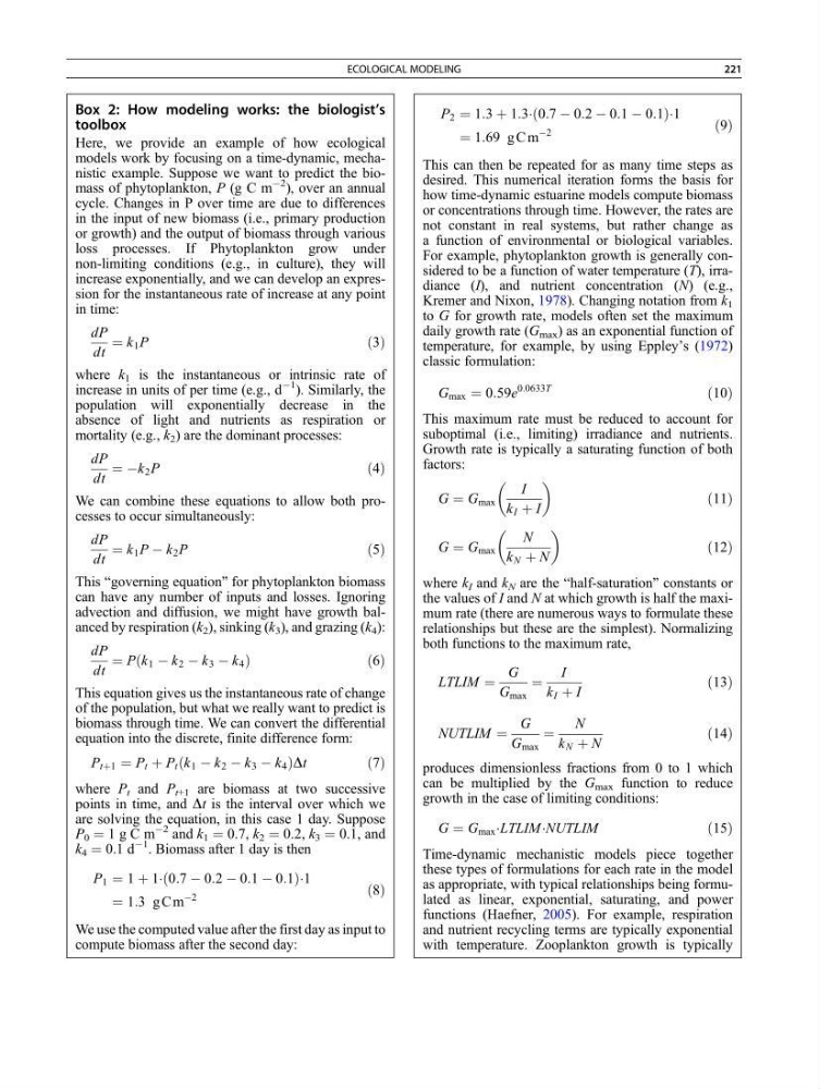
Box 2: How modeling works: the biologist’s
toolbox
Here, we provide an example of how ecological
models work by focusing on a time-dynamic, mechanistic example. Suppose we want to predict the biomass of phytoplankton, P (g C m
À2
), over an annual
cycle. Changes in P over time are due to differences
in the input of new biomass (i.e., primary production
or growth) and the output of biomass through various
loss processes. If Phytoplankton grow under
non-limiting conditions (e.g., in culture), they will
increase exponentially, and we can develop an expression for the instantaneous rate of increase at any point
in time:
dP
dt
¼ k 1 P
ð3Þ
where k 1 is the instantaneous or intrinsic rate of
increase in units of per time (e.g., d
À1
). Similarly, the
population will exponentially decrease in the
absence of light and nutrients as respiration or
mortality (e.g., k 2 ) are the dominant processes:
dP
dt
¼ Àk 2 P
ð4Þ
We can combine these equations to allow both processes to occur simultaneously:
dP
dt
¼ k 1 P À k 2 P
ð5Þ
This “governing equation” for phytoplankton biomass
can have any number of inputs and losses. Ignoring
advection and diffusion, we might have growth balanced by respiration (k 2 ), sinking (k 3 ), and grazing (k 4 ):
dP
dt
¼ P k 1 À k 2 À k 3 À k 4
ð
Þ
ð 6Þ
This equation gives us the instantaneous rate of change
of the population, but what we really want to predict is
biomass through time. We can convert the differential
equation into the discrete, finite difference form:
P tþ1 ¼ P t þ P t k 1 À k 2 À k 3 À k 4
ð
Þ Dt
ð7Þ
where P t and P t+1 are biomass at two successive
points in time, and Dt is the interval over which we
are solving the equation, in this case 1 day. Suppose
P 0 ¼ 1 g C m
À2 and k 1 ¼ 0.7, k 2 ¼ 0.2, k 3 ¼ 0.1, and
k 4 ¼ 0.1 d
À1
. Biomass after 1 day is then
P 1 ¼ 1 þ 1Á 0:7 À 0:2 À 0:1 À 0:1
ð
Þ Á 1
¼ 1:3 gCm
À2
ð8Þ
We use the computed value after the first day as input to
compute biomass after the second day:
P 2 ¼ 1:3 þ 1:3Á 0:7 À 0:2 À 0:1 À 0:1
ð
Þ Á 1
¼ 1:69 g C m
À2
ð9Þ
This can then be repeated for as many time steps as
desired. This numerical iteration forms the basis for
how time-dynamic estuarine models compute biomass
or concentrations through time. However, the rates are
not constant in real systems, but rather change as
a function of environmental or biological variables.
For example, phytoplankton growth is generally considered to be a function of water temperature (T), irradiance (I), and nutrient concentration (N) (e.g.,
Kremer and Nixon, 1978). Changing notation from k 1
to G for growth rate, models often set the maximum
daily growth rate (G max ) as an exponential function of
temperature, for example, by using Eppley’s (1972)
classic formulation:
G max ¼ 0:59e
0:0633T
ð10Þ
This maximum rate must be reduced to account for
suboptimal (i.e., limiting) irradiance and nutrients.
Growth rate is typically a saturating function of both
factors:
G ¼ G max
I
k I þ I
ð11Þ
G ¼ G max
N
k N þ N
ð12Þ
where k I and k N are the “half-saturation” constants or
the values of I and N at which growth is half the maximum rate (there are numerous ways to formulate these
relationships but these are the simplest). Normalizing
both functions to the maximum rate,
LTLIM ¼
G
G max
¼
I
k I þ I
ð13Þ
NUTLIM ¼
G
G max
¼
N
k N þ N
ð14Þ
produces dimensionless fractions from 0 to 1 which
can be multiplied by the G max function to reduce
growth in the case of limiting conditions:
G ¼ G max ÁLTLIM ÁNUTLIM
ð15Þ
Time-dynamic mechanistic models piece together
these types of formulations for each rate in the model
as appropriate, with typical relationships being formulated as linear, exponential, saturating, and power
functions (Haefner, 2005). For example, respiration
and nutrient recycling terms are typically exponential
with temperature. Zooplankton growth is typically
ECOLOGICAL MODELING
221
toolbox
Here, we provide an example of how ecological
models work by focusing on a time-dynamic, mechanistic example. Suppose we want to predict the biomass of phytoplankton, P (g C m
À2
), over an annual
cycle. Changes in P over time are due to differences
in the input of new biomass (i.e., primary production
or growth) and the output of biomass through various
loss processes. If Phytoplankton grow under
non-limiting conditions (e.g., in culture), they will
increase exponentially, and we can develop an expression for the instantaneous rate of increase at any point
in time:
dP
dt
¼ k 1 P
ð3Þ
where k 1 is the instantaneous or intrinsic rate of
increase in units of per time (e.g., d
À1
). Similarly, the
population will exponentially decrease in the
absence of light and nutrients as respiration or
mortality (e.g., k 2 ) are the dominant processes:
dP
dt
¼ Àk 2 P
ð4Þ
We can combine these equations to allow both processes to occur simultaneously:
dP
dt
¼ k 1 P À k 2 P
ð5Þ
This “governing equation” for phytoplankton biomass
can have any number of inputs and losses. Ignoring
advection and diffusion, we might have growth balanced by respiration (k 2 ), sinking (k 3 ), and grazing (k 4 ):
dP
dt
¼ P k 1 À k 2 À k 3 À k 4
ð
Þ
ð 6Þ
This equation gives us the instantaneous rate of change
of the population, but what we really want to predict is
biomass through time. We can convert the differential
equation into the discrete, finite difference form:
P tþ1 ¼ P t þ P t k 1 À k 2 À k 3 À k 4
ð
Þ Dt
ð7Þ
where P t and P t+1 are biomass at two successive
points in time, and Dt is the interval over which we
are solving the equation, in this case 1 day. Suppose
P 0 ¼ 1 g C m
À2 and k 1 ¼ 0.7, k 2 ¼ 0.2, k 3 ¼ 0.1, and
k 4 ¼ 0.1 d
À1
. Biomass after 1 day is then
P 1 ¼ 1 þ 1Á 0:7 À 0:2 À 0:1 À 0:1
ð
Þ Á 1
¼ 1:3 gCm
À2
ð8Þ
We use the computed value after the first day as input to
compute biomass after the second day:
P 2 ¼ 1:3 þ 1:3Á 0:7 À 0:2 À 0:1 À 0:1
ð
Þ Á 1
¼ 1:69 g C m
À2
ð9Þ
This can then be repeated for as many time steps as
desired. This numerical iteration forms the basis for
how time-dynamic estuarine models compute biomass
or concentrations through time. However, the rates are
not constant in real systems, but rather change as
a function of environmental or biological variables.
For example, phytoplankton growth is generally considered to be a function of water temperature (T), irradiance (I), and nutrient concentration (N) (e.g.,
Kremer and Nixon, 1978). Changing notation from k 1
to G for growth rate, models often set the maximum
daily growth rate (G max ) as an exponential function of
temperature, for example, by using Eppley’s (1972)
classic formulation:
G max ¼ 0:59e
0:0633T
ð10Þ
This maximum rate must be reduced to account for
suboptimal (i.e., limiting) irradiance and nutrients.
Growth rate is typically a saturating function of both
factors:
G ¼ G max
I
k I þ I
ð11Þ
G ¼ G max
N
k N þ N
ð12Þ
where k I and k N are the “half-saturation” constants or
the values of I and N at which growth is half the maximum rate (there are numerous ways to formulate these
relationships but these are the simplest). Normalizing
both functions to the maximum rate,
LTLIM ¼
G
G max
¼
I
k I þ I
ð13Þ
NUTLIM ¼
G
G max
¼
N
k N þ N
ð14Þ
produces dimensionless fractions from 0 to 1 which
can be multiplied by the G max function to reduce
growth in the case of limiting conditions:
G ¼ G max ÁLTLIM ÁNUTLIM
ð15Þ
Time-dynamic mechanistic models piece together
these types of formulations for each rate in the model
as appropriate, with typical relationships being formulated as linear, exponential, saturating, and power
functions (Haefner, 2005). For example, respiration
and nutrient recycling terms are typically exponential
with temperature. Zooplankton growth is typically
ECOLOGICAL MODELING
221