

Types of models
At the most basic level, models can be divided into conceptual and mathematical models (Figure 3). The former present a diagrammatic synthesis of the interrelationships
between components of an estuary and allow one to draw
qualitative predictions about how a system will respond to
perturbation. Mathematical models do the same, except that
the relationships are formulated with equations to allow
quantitative prediction. Mathematical models can be
divided into empirical and mechanistic models; the former
are statistical relationships between variables which can
often provide powerful predictive capability. Classic examples for aquatic systems include the phosphorus-chlorophyll
models of Dillon and Rigler (1974) and Vollenweider
(1976) for lakes, which have been extended into estuaries
using nitrogen as the limiting nutrient and chlorophyll,
primary production, and fisheries yields as the response variables (e.g., Nixon, 1992; Boynton and Kemp, 2000; Nixon
et al., 2001). However, statistical models do not provide
any underlying explanation of the processes involved
(i.e., “correlation does not imply causation”).
Mechanistic or process models attempt to provide this
explanation by developing equations that piece together
individual physiological, ecological, and behavioral formulations that relate ecological rates (e.g., growth, consumption, respiration) to environmental or biological
factors (e.g., biomass, temperature, light, nutrients). Some
mechanistic models are simple enough that exact analytical solutions can be determined through integration (i.e.,
an exact estimate of biomass or concentration at any future
time). However, most are too complex for an exact analytical solution and must be solved over successive time
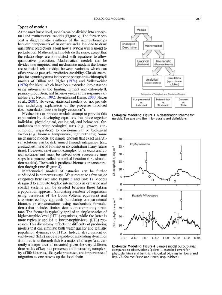
steps in a process called numerical iteration (i.e., simulation models). The result is predicted biomass or concentration through time (Figure 4).
Mathematical models of estuaries can be further
subdivided in numerous ways. We summarize a few major
categories here (see also Figure 3 and Box 1). Models
designed to simulate trophic interactions in estuarine and
coastal systems can be divided between those taking
a population approach (simulating numbers of organisms
using variations of the Lotka-Volterra equations) and
a systems ecology approach (simulating compartmental
biomass or concentrations using mechanistic formulations) that includes limited details on community structure. The former is typically applied to single species of
higher-trophic-level (HTL) organisms, while the latter is
more typically applied to lower-trophic-level (LTL) processes. This dichotomy reflects the difficulty of producing
models that can simulate both water quality and realistic
population dynamics of HTLs. Indeed, development of
end-to-end (E2E) models capable of simulating dynamics
from nutrients through fish is a major challenge (and currently a major area of research) given the very different
time scales of key rate processes and increasing complexity of life histories, life cycle processes, and importance of
migration as one moves up the food chain.
Ecological Modeling, Figure 3 A classification scheme for
models. See text and Box 1 for details and definitions.
Ecological Modeling, Figure 4 Sample model output (lines)
compared to observations (points Æ standard error) for
phytoplankton and benthic microalgal biomass in Hog Island
Bay, VA (Source: Brush and Harris, unpublished).
ECOLOGICAL MODELING
217
At the most basic level, models can be divided into conceptual and mathematical models (Figure 3). The former present a diagrammatic synthesis of the interrelationships
between components of an estuary and allow one to draw
qualitative predictions about how a system will respond to
perturbation. Mathematical models do the same, except that
the relationships are formulated with equations to allow
quantitative prediction. Mathematical models can be
divided into empirical and mechanistic models; the former
are statistical relationships between variables which can
often provide powerful predictive capability. Classic examples for aquatic systems include the phosphorus-chlorophyll
models of Dillon and Rigler (1974) and Vollenweider
(1976) for lakes, which have been extended into estuaries
using nitrogen as the limiting nutrient and chlorophyll,
primary production, and fisheries yields as the response variables (e.g., Nixon, 1992; Boynton and Kemp, 2000; Nixon
et al., 2001). However, statistical models do not provide
any underlying explanation of the processes involved
(i.e., “correlation does not imply causation”).
Mechanistic or process models attempt to provide this
explanation by developing equations that piece together
individual physiological, ecological, and behavioral formulations that relate ecological rates (e.g., growth, consumption, respiration) to environmental or biological
factors (e.g., biomass, temperature, light, nutrients). Some
mechanistic models are simple enough that exact analytical solutions can be determined through integration (i.e.,
an exact estimate of biomass or concentration at any future
time). However, most are too complex for an exact analytical solution and must be solved over successive time
steps in a process called numerical iteration (i.e., simulation models). The result is predicted biomass or concentration through time (Figure 4).
Mathematical models of estuaries can be further
subdivided in numerous ways. We summarize a few major
categories here (see also Figure 3 and Box 1). Models
designed to simulate trophic interactions in estuarine and
coastal systems can be divided between those taking
a population approach (simulating numbers of organisms
using variations of the Lotka-Volterra equations) and
a systems ecology approach (simulating compartmental
biomass or concentrations using mechanistic formulations) that includes limited details on community structure. The former is typically applied to single species of
higher-trophic-level (HTL) organisms, while the latter is
more typically applied to lower-trophic-level (LTL) processes. This dichotomy reflects the difficulty of producing
models that can simulate both water quality and realistic
population dynamics of HTLs. Indeed, development of
end-to-end (E2E) models capable of simulating dynamics
from nutrients through fish is a major challenge (and currently a major area of research) given the very different
time scales of key rate processes and increasing complexity of life histories, life cycle processes, and importance of
migration as one moves up the food chain.
Ecological Modeling, Figure 3 A classification scheme for
models. See text and Box 1 for details and definitions.
Ecological Modeling, Figure 4 Sample model output (lines)
compared to observations (points Æ standard error) for
phytoplankton and benthic microalgal biomass in Hog Island
Bay, VA (Source: Brush and Harris, unpublished).
ECOLOGICAL MODELING
217