

18
J.L. Giraudel . S. Lek
2.2.2
The Self-Organizing Map (SOM) Aigorithm
This section explains how the SOM algorithm can be adapted to an abundance
dataset. The SOM algorithm has been described by Kohonen (1982) in the early
eighties. Since that time, it has been most widely used for data mining and
knowledge discovery.
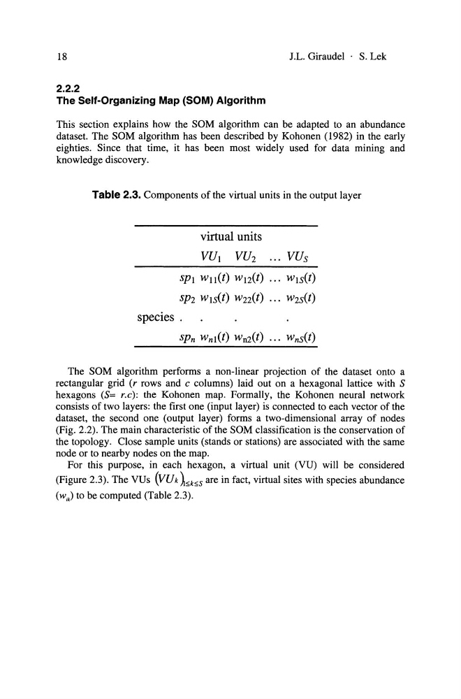
Table 2.3. Components of the virtual units in the output layer
virtual units
VU1 VU2
VUs
SPI Wl1(t) W12(t)
SP2 WlS(t) W22(t)
species .
sPn Wnl(t) Wn2(t)
The SOM algorithm perforrns a non-linear projection of the dataset onto a
rectangular grid (r rows and c columns) laid out on a hexagonal lattice with S
hexagons (S= r.c): the Kohonen map. Formally, the Kohonen neural network
consists of two layers: the first one (input layer) is connected to each vector of the
dataset, the second one (output layer) forms a two-dimensional array of nodes
(Fig. 2.2). The main characteristic of the SOM classification is the conservation of
the topology. Close sampie units (stands or stations) are associated with the same
node or to nearby nodes on the map.
For this purpose, in each hexagon, a virtual unit (VU) will be considered
(Figure 2.3). The VUs (VUk A!>k!>S are in fact, virtual sites with species abundance
(W;k) to be computed (Table 2.3).
J.L. Giraudel . S. Lek
2.2.2
The Self-Organizing Map (SOM) Aigorithm
This section explains how the SOM algorithm can be adapted to an abundance
dataset. The SOM algorithm has been described by Kohonen (1982) in the early
eighties. Since that time, it has been most widely used for data mining and
knowledge discovery.
Table 2.3. Components of the virtual units in the output layer
virtual units
VU1 VU2
VUs
SPI Wl1(t) W12(t)
SP2 WlS(t) W22(t)
species .
sPn Wnl(t) Wn2(t)
The SOM algorithm perforrns a non-linear projection of the dataset onto a
rectangular grid (r rows and c columns) laid out on a hexagonal lattice with S
hexagons (S= r.c): the Kohonen map. Formally, the Kohonen neural network
consists of two layers: the first one (input layer) is connected to each vector of the
dataset, the second one (output layer) forms a two-dimensional array of nodes
(Fig. 2.2). The main characteristic of the SOM classification is the conservation of
the topology. Close sampie units (stands or stations) are associated with the same
node or to nearby nodes on the map.
For this purpose, in each hexagon, a virtual unit (VU) will be considered
(Figure 2.3). The VUs (VUk A!>k!>S are in fact, virtual sites with species abundance
(W;k) to be computed (Table 2.3).