

388
G.M.Foody
adjusted in relation to the error magnitude. Typically the weight adjustment is
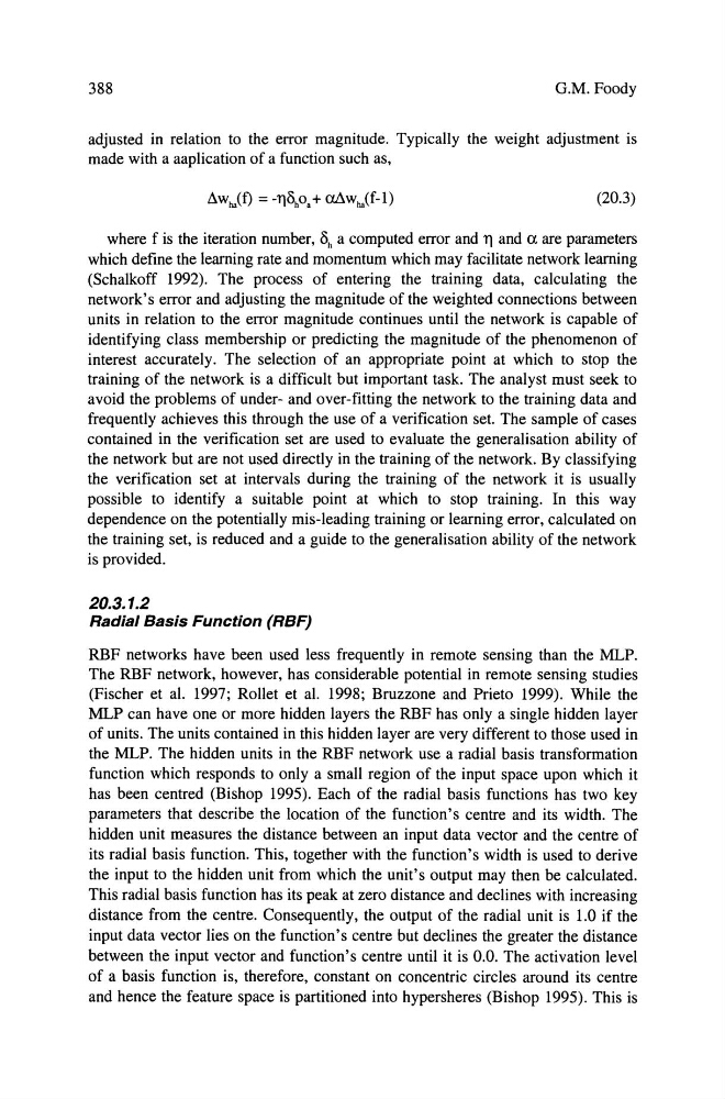
made with a aaplication of a function such as,
(20.3)
where fis the iteration number, 0h a computed error and 11 and a are parameters
which define the leaming rate and momentum which may facilitate network leaming
(Schalkoff 1992). The process of entering the training data, calculating the
network's error and adjusting the magnitude of the weighted connections between
units in relation to the error magnitude continues until the network is capable of
identifying cIass membership or predicting the magnitude of the phenomenon of
interest accurately. The selection of an appropriate point at which to stop the
training of the network is a difficult but important task. The analyst must seek to
avoid the problems of under- and over-fitting the network to the training data and
frequently achieves this through the use of a verification set. The sampie of cases
contained in the verification set are used to evaluate the generalisation ability of
the network but are not used directly in the training of the network. By cIassifying
the verification set at intervals during the training of the network it is usually
possible to identify a suitable point at wh ich to stop training. In this way
dependence on the potentially mis-leading training or leaming error, calculated on
the training set, is reduced and a guide to the generalisation ability of the network
is provided.
20.3.1.2
Radial Basis Function (RBF)
RBF networks have been used less frequently in remote sensing than the MLP.
The RBF network, however, has considerable potential in remote sensing studies
(Fischer et al. 1997; Rollet et al. 1998; Bruzzone and Prieto 1999). While the
MLP can have one or more hidden layers the RBF has only a single hidden layer
of units. The units contained in this hidden layer are very different to those used in
the MLP. The hidden units in the RBF network use a radial basis transformation
function which responds to only a small region of the input space upon which it
has been centred (Bishop 1995). Each of the radial basis functions has two key
parameters that describe the location of the function's centre and its width. The
hidden unit measures the distance between an input data vector and the centre of
its radial basis function. This, together with the function's width is used to derive
the input to the hidden unit from which the unit's output may then be calculated.
This radial basis function has its peak at zero distance and decIines with increasing
distance from the centre. Consequently, the output of the radial unit is 1.0 if the
input data vector lies on the function's centre but decIines the greater the distance
between the input vector and function's centre until it is 0.0. The activation level
of a basis function is, therefore, constant on concentric circIes around its centre
and hence the feature space is partitioned into hypersheres (Bishop 1995). This is
G.M.Foody
adjusted in relation to the error magnitude. Typically the weight adjustment is
made with a aaplication of a function such as,
(20.3)
where fis the iteration number, 0h a computed error and 11 and a are parameters
which define the leaming rate and momentum which may facilitate network leaming
(Schalkoff 1992). The process of entering the training data, calculating the
network's error and adjusting the magnitude of the weighted connections between
units in relation to the error magnitude continues until the network is capable of
identifying cIass membership or predicting the magnitude of the phenomenon of
interest accurately. The selection of an appropriate point at which to stop the
training of the network is a difficult but important task. The analyst must seek to
avoid the problems of under- and over-fitting the network to the training data and
frequently achieves this through the use of a verification set. The sampie of cases
contained in the verification set are used to evaluate the generalisation ability of
the network but are not used directly in the training of the network. By cIassifying
the verification set at intervals during the training of the network it is usually
possible to identify a suitable point at wh ich to stop training. In this way
dependence on the potentially mis-leading training or leaming error, calculated on
the training set, is reduced and a guide to the generalisation ability of the network
is provided.
20.3.1.2
Radial Basis Function (RBF)
RBF networks have been used less frequently in remote sensing than the MLP.
The RBF network, however, has considerable potential in remote sensing studies
(Fischer et al. 1997; Rollet et al. 1998; Bruzzone and Prieto 1999). While the
MLP can have one or more hidden layers the RBF has only a single hidden layer
of units. The units contained in this hidden layer are very different to those used in
the MLP. The hidden units in the RBF network use a radial basis transformation
function which responds to only a small region of the input space upon which it
has been centred (Bishop 1995). Each of the radial basis functions has two key
parameters that describe the location of the function's centre and its width. The
hidden unit measures the distance between an input data vector and the centre of
its radial basis function. This, together with the function's width is used to derive
the input to the hidden unit from which the unit's output may then be calculated.
This radial basis function has its peak at zero distance and decIines with increasing
distance from the centre. Consequently, the output of the radial unit is 1.0 if the
input data vector lies on the function's centre but decIines the greater the distance
between the input vector and function's centre until it is 0.0. The activation level
of a basis function is, therefore, constant on concentric circIes around its centre
and hence the feature space is partitioned into hypersheres (Bishop 1995). This is