

Chapter 17· Classification of Fish Stock-Recruitment Relationships 331
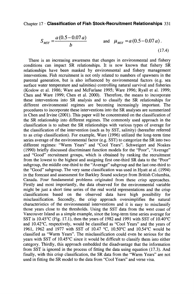
s = a(O.5-0.07 a)
MSY
b
and J1MSY =a(O.5-0.07 a).
(17.4)
There is an increasing awareness that changes in environmental and fishery
conditions can impact SR relationships. It is now known that fishery SR
relationships have been masked by environmental and fishery management
interventions. Fish recruitment is not only related to numbers of spawners in the
parental generation, but is also influenced by environmental factors (e.g. sea
surface water temperature and salinities) controlling natural survival and fisheries
(Koslow et al. 1986; Ware and McFarlane 1995; Ware 1996; Ryall et al. 1999;
Chen and Ware 1999; Chen et al. 2000). Therefore, the means to incorporate
these interventions into SR analysis and to classify the SR relationships for
different environmental regimes are becoming increasingly important. The
procedures to incorporate these interventions into the SR analyses are summerized
in Chen and Irvine (2001). This paper will be concentrated on the classification of
the SR relationship into different regimes. The commonly used approach in the
classification is to sub set the SR relationships with various types of average for
the classification of the intervention (such as by SST, salinity) (hereafter referred
to as crisp classification). For example, Ware (1996) utilized the long-term time
series average of the environmental factor (e.g. SST) to categorize the SR into two
different regimes: "Warm Years" and "Cool Years". Schweigert and Noakes
(1990) briefly discussed discriminant function models for the "Poor", "Average"
and "Good" recruitment groups, which is obtained by ranking the recruitment
from the lowest to the highest and assigning first one-third SR data to the "Poor"
subgroup, the middle one-third to the "Average" subgroup and the last one-third to
the "Good" subgroup. The very same classification was used in Hyatt at al. (1994)
in the forecast and assessment for Barkley Sound sockeye from British Columbia,
Canada. Four fundamental problems originated from these crisp approaches.
Firstly and most importantly, the data observed for the environmental variable
might be just a short time series of the real world representations and the crisp
classifications based on the observed data have high possibility for
misclassification. Secondly, the crisp approach oversimplifies the natural
characteristics of the environmental interventions and it is easy to misclassify
those years close to the thresholds. Using the SST data from the west co ast of
Vancouver Island as a simple example, since the long-term time series average for
SST is 1O.45°C (Fig. 17.1), then the years of 1982 and 1991 with SST of 10.40OC
and 1O.42°C, respectively, would be classified as "Cool Years" and the years of
1961, 1962 and 1977 with SST of 10.47 °C, 10.50°C and 1O.54°C would be
classified as "Warm Years". The misclassification could even be serious for the
years with SST of 1O.45°C since it would be difficult to classify them into either
category. Thirdly, this approach embedded the dis advantage that the information
from SST is ignored in the process of fitting the data using equation (17.3). And
finally, with this crisp classification, the SR data from the "Warm Years" are not
used in fitting the SR model to the data from "Cool Years" and verse visa.
s = a(O.5-0.07 a)
MSY
b
and J1MSY =a(O.5-0.07 a).
(17.4)
There is an increasing awareness that changes in environmental and fishery
conditions can impact SR relationships. It is now known that fishery SR
relationships have been masked by environmental and fishery management
interventions. Fish recruitment is not only related to numbers of spawners in the
parental generation, but is also influenced by environmental factors (e.g. sea
surface water temperature and salinities) controlling natural survival and fisheries
(Koslow et al. 1986; Ware and McFarlane 1995; Ware 1996; Ryall et al. 1999;
Chen and Ware 1999; Chen et al. 2000). Therefore, the means to incorporate
these interventions into SR analysis and to classify the SR relationships for
different environmental regimes are becoming increasingly important. The
procedures to incorporate these interventions into the SR analyses are summerized
in Chen and Irvine (2001). This paper will be concentrated on the classification of
the SR relationship into different regimes. The commonly used approach in the
classification is to sub set the SR relationships with various types of average for
the classification of the intervention (such as by SST, salinity) (hereafter referred
to as crisp classification). For example, Ware (1996) utilized the long-term time
series average of the environmental factor (e.g. SST) to categorize the SR into two
different regimes: "Warm Years" and "Cool Years". Schweigert and Noakes
(1990) briefly discussed discriminant function models for the "Poor", "Average"
and "Good" recruitment groups, which is obtained by ranking the recruitment
from the lowest to the highest and assigning first one-third SR data to the "Poor"
subgroup, the middle one-third to the "Average" subgroup and the last one-third to
the "Good" subgroup. The very same classification was used in Hyatt at al. (1994)
in the forecast and assessment for Barkley Sound sockeye from British Columbia,
Canada. Four fundamental problems originated from these crisp approaches.
Firstly and most importantly, the data observed for the environmental variable
might be just a short time series of the real world representations and the crisp
classifications based on the observed data have high possibility for
misclassification. Secondly, the crisp approach oversimplifies the natural
characteristics of the environmental interventions and it is easy to misclassify
those years close to the thresholds. Using the SST data from the west co ast of
Vancouver Island as a simple example, since the long-term time series average for
SST is 1O.45°C (Fig. 17.1), then the years of 1982 and 1991 with SST of 10.40OC
and 1O.42°C, respectively, would be classified as "Cool Years" and the years of
1961, 1962 and 1977 with SST of 10.47 °C, 10.50°C and 1O.54°C would be
classified as "Warm Years". The misclassification could even be serious for the
years with SST of 1O.45°C since it would be difficult to classify them into either
category. Thirdly, this approach embedded the dis advantage that the information
from SST is ignored in the process of fitting the data using equation (17.3). And
finally, with this crisp classification, the SR data from the "Warm Years" are not
used in fitting the SR model to the data from "Cool Years" and verse visa.