

6.7 Variance of Estimators Derived from the Horvitz-Thompson Estimator
87
start, and the remaining cells are located at intervals of m cells from each other. Figure 6.1 shows
plot locations from a systematic sampling design
of this type. Under this design, the inclusion probabilities are 7T; = 1I(km) for each of the i cells in
the lattice population. For example, if we choose
every third lattice point to start a transect and every
other cell on each transect, then the inclusion Pfobabilities for the sample units are all equal to 6'
A design that illustrates cluster sampling of the
lattice population begins by choosing an SRS of n
cells. Each cell in the SRS defines a cluster center,
and the clusters are defined to be sets of k > 1 contiguous cells centered about the cluster center and
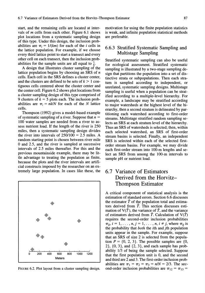
the center cell. Figure 6.2 shows plot locations from
a cluster sampling design of this type comprised of
9 clusters of k = 5 plots each. The inclusion probabilities are 7T; = nklN for each of the N lattice
cells.
Thompson (1992) gives a model-based example
of systematic sampling of a river. Suppose that n =
100 water samples are needed from a river to assess nutrient load. If the length of the river is 250
miles, then a systematic sampling design divides
the river into intervals of 250/100 = 2.5 miles. A
random starting point is chosen between river mile
° and 2.5, and the river is sampled at successive
intervals of 2.5 miles thereafter. For this and the
previous mountainside example, there may be little advantage to treating the population as finite,
because the plots and the river intervals are artificial constructs imposed by the researcher on an extremely large population. In cases like these, the
o&qp
0&
,0&
,
0
200
400
600
800
1000 1200
Meters
FiGURE 6.2. Plot layout from a cluster sampling design.
motivation for using the finite population statistics
is weak, and infinite population statistical methods
are preferable.
6.6.3 Stratified Systematic Sampling and
Multistage Sampling
Stratified systematic sampling can also be useful
for ecological assessment. Stratified systematic
sampling is illustrated by a two-stage sampling design that partitions the population into a set of distinctive strata or subpopulations. Then each stratum is sampled according to independent, or
unrelated, systematic sampling designs. Multistage
sampling is useful when a population can be stratified according to a multiple-level hierarchy. For
example, a landscape may be stratified according
to major watersheds at the highest level of the hierarchy, then a second stratum is delineated by partitioning each watershed according to first-order
streams. Multistage stratified random sampling selects an SRS at each stratum level of the hierarchy.
Thus an SRS of watersheds is selected; then, within
each selected watershed, an SRS of first-order
stream basins is selected. Finally, an independent
SRS is selected within each of the selected firstorder stream basins. For example, we may divide
each first-order stream into 100-m lengths and select an SRS from among the 100-m intervals to
sample pH or nutrient load.
6.7 Variance of Estimators
Derived from the HorvitzThompson Estimator
A critical component of statistical analysis is the
estimation of standard errors. Section 6.6 discusses
the estimator t of the population total and estimators derived from t. This section discusses estimation of V (T), the variance~ of t, and the varians.e
of estimators derived from T. Calculation of V(D
requires the second-order inclusion probabilities
7Tij, i = 1, ... , n, j = 1, ... , n, i *- j, where 7Tij is
the probability that both the ith and jth population
units appear in the sample. For example, suppose
that an SRS of size 2 is selected from the population P = {O, 2, 3}. The possible samples are {O,
2}, {O, 3}, and {2, 3}, and each sample has probability 113 of being the sample selected. Suppose
that the first population unit is 0, and the second
and third are 2 and 3. The first-order inclusion probabilities are 7Tl = 7T2 = 7T3 = nlN = 2/3. The second-order inclusion probabilities are 7Tl2 = 7T13 =
87
start, and the remaining cells are located at intervals of m cells from each other. Figure 6.1 shows
plot locations from a systematic sampling design
of this type. Under this design, the inclusion probabilities are 7T; = 1I(km) for each of the i cells in
the lattice population. For example, if we choose
every third lattice point to start a transect and every
other cell on each transect, then the inclusion Pfobabilities for the sample units are all equal to 6'
A design that illustrates cluster sampling of the
lattice population begins by choosing an SRS of n
cells. Each cell in the SRS defines a cluster center,
and the clusters are defined to be sets of k > 1 contiguous cells centered about the cluster center and
the center cell. Figure 6.2 shows plot locations from
a cluster sampling design of this type comprised of
9 clusters of k = 5 plots each. The inclusion probabilities are 7T; = nklN for each of the N lattice
cells.
Thompson (1992) gives a model-based example
of systematic sampling of a river. Suppose that n =
100 water samples are needed from a river to assess nutrient load. If the length of the river is 250
miles, then a systematic sampling design divides
the river into intervals of 250/100 = 2.5 miles. A
random starting point is chosen between river mile
° and 2.5, and the river is sampled at successive
intervals of 2.5 miles thereafter. For this and the
previous mountainside example, there may be little advantage to treating the population as finite,
because the plots and the river intervals are artificial constructs imposed by the researcher on an extremely large population. In cases like these, the
o&qp
0&
,0&
,
0
200
400
600
800
1000 1200
Meters
FiGURE 6.2. Plot layout from a cluster sampling design.
motivation for using the finite population statistics
is weak, and infinite population statistical methods
are preferable.
6.6.3 Stratified Systematic Sampling and
Multistage Sampling
Stratified systematic sampling can also be useful
for ecological assessment. Stratified systematic
sampling is illustrated by a two-stage sampling design that partitions the population into a set of distinctive strata or subpopulations. Then each stratum is sampled according to independent, or
unrelated, systematic sampling designs. Multistage
sampling is useful when a population can be stratified according to a multiple-level hierarchy. For
example, a landscape may be stratified according
to major watersheds at the highest level of the hierarchy, then a second stratum is delineated by partitioning each watershed according to first-order
streams. Multistage stratified random sampling selects an SRS at each stratum level of the hierarchy.
Thus an SRS of watersheds is selected; then, within
each selected watershed, an SRS of first-order
stream basins is selected. Finally, an independent
SRS is selected within each of the selected firstorder stream basins. For example, we may divide
each first-order stream into 100-m lengths and select an SRS from among the 100-m intervals to
sample pH or nutrient load.
6.7 Variance of Estimators
Derived from the HorvitzThompson Estimator
A critical component of statistical analysis is the
estimation of standard errors. Section 6.6 discusses
the estimator t of the population total and estimators derived from t. This section discusses estimation of V (T), the variance~ of t, and the varians.e
of estimators derived from T. Calculation of V(D
requires the second-order inclusion probabilities
7Tij, i = 1, ... , n, j = 1, ... , n, i *- j, where 7Tij is
the probability that both the ith and jth population
units appear in the sample. For example, suppose
that an SRS of size 2 is selected from the population P = {O, 2, 3}. The possible samples are {O,
2}, {O, 3}, and {2, 3}, and each sample has probability 113 of being the sample selected. Suppose
that the first population unit is 0, and the second
and third are 2 and 3. The first-order inclusion probabilities are 7Tl = 7T2 = 7T3 = nlN = 2/3. The second-order inclusion probabilities are 7Tl2 = 7T13 =