

46
Ecosystem Characterization and Ecological Assessments
EXAMPLE:ABUVVASC
CD
®
®
en
....
CU
~
10 7
I
I
i
i
10 6
i
!
!
10 5
10 4
10 3
10 2
10 1
10 2
ABLA = SUBALPINE FIR
Meters 2
PI CO = LODGEPOLE PINE
VASC = GROUSE WHORTLEBERRY
{D®or@
,,..-I Cnmate ~\ ~
.~Vegetation type~ •• ,,"'" r - - - - - ,
.--------, •••• :. Terrestrial or
~ Landform type f··... Aquatic
ECOLOGICAL
.j Soil type ~ •..• '
LAND
.""
UNIT
• ., Hydroregime
.,.~ Rock type
1··:::/1-..---.-----1
f' "
!
1+~~~~~"I_Classification---""_---IEvaluationl---_'1
_._.- Observation
.•...••..•. Classification
- - Evaluation
Reference base
for evaluation
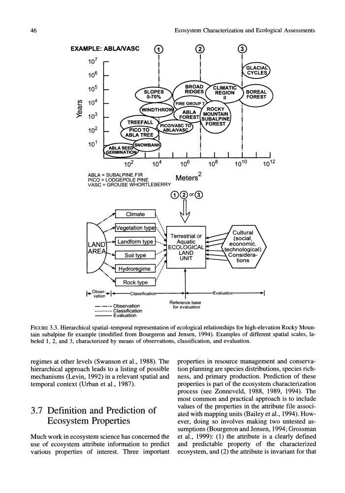
FIGURE 3.3. Hierarchical spatial-temporal representation of ecological relationships for high-elevation Rocky Mountain subalpine fir example (modified from Bourgeron and Jensen, 1994). Examples of different spatial scales, labeled 1, 2, and 3, characterized by means of observations, classification, and evaluation.
regimes at other levels (Swanson et al., 1988). The
hierarchical approach leads to a listing of possible
mechanisms (Levin, 1992) in a relevant spatial and
temporal context (Urban et al., 1987).
3.7 Definition and Prediction of
Ecosystem Properties
Much work in ecosystem science has concerned the
use of ecosystem attribute information to predict
various properties of interest. Three important
properties in resource management and conservation planning are species distributions, species richness, and primary production. Prediction of these
properties is part of the ecosystem characterization
process (see Zonneveld, 1988, 1989, 1994). The
most common and practical approach is to include
values of the properties in the attribute file associated with mapping units (Bailey et al., 1994). However, doing so involves making two untested assumptions (Bourgeron and Jensen, 1994; Grossman
et al., 1999): (1) the attribute is a clearly defined
and predictable property of the characterized
ecosystem, and (2) the attribute is invariant for that
Ecosystem Characterization and Ecological Assessments
EXAMPLE:ABUVVASC
CD
®
®
en
....
CU
~
10 7
I
I
i
i
10 6
i
!
!
10 5
10 4
10 3
10 2
10 1
10 2
ABLA = SUBALPINE FIR
Meters 2
PI CO = LODGEPOLE PINE
VASC = GROUSE WHORTLEBERRY
{D®or@
,,..-I Cnmate ~\ ~
.~Vegetation type~ •• ,,"'" r - - - - - ,
.--------, •••• :. Terrestrial or
~ Landform type f··... Aquatic
ECOLOGICAL
.j Soil type ~ •..• '
LAND
.""
UNIT
• ., Hydroregime
.,.~ Rock type
1··:::/1-..---.-----1
f' "
!
1+~~~~~"I_Classification---""_---IEvaluationl---_'1
_._.- Observation
.•...••..•. Classification
- - Evaluation
Reference base
for evaluation
FIGURE 3.3. Hierarchical spatial-temporal representation of ecological relationships for high-elevation Rocky Mountain subalpine fir example (modified from Bourgeron and Jensen, 1994). Examples of different spatial scales, labeled 1, 2, and 3, characterized by means of observations, classification, and evaluation.
regimes at other levels (Swanson et al., 1988). The
hierarchical approach leads to a listing of possible
mechanisms (Levin, 1992) in a relevant spatial and
temporal context (Urban et al., 1987).
3.7 Definition and Prediction of
Ecosystem Properties
Much work in ecosystem science has concerned the
use of ecosystem attribute information to predict
various properties of interest. Three important
properties in resource management and conservation planning are species distributions, species richness, and primary production. Prediction of these
properties is part of the ecosystem characterization
process (see Zonneveld, 1988, 1989, 1994). The
most common and practical approach is to include
values of the properties in the attribute file associated with mapping units (Bailey et al., 1994). However, doing so involves making two untested assumptions (Bourgeron and Jensen, 1994; Grossman
et al., 1999): (1) the attribute is a clearly defined
and predictable property of the characterized
ecosystem, and (2) the attribute is invariant for that